
Solution by Separation of Variables
Enroll to start learning
You’ve not yet enrolled in this course. Please enroll for free to listen to audio lessons, classroom podcasts and take practice test.
Interactive Audio Lesson
Listen to a student-teacher conversation explaining the topic in a relatable way.
Introduction to Separation of Variables
🔒 Unlock Audio Lesson
Sign up and enroll to listen to this audio lesson

Today, we're going to explore the method of separation of variables. It's a powerful tool for solving partial differential equations like the one we have in the two-dimensional wave equation. Can anyone tell me how we would start with such an equation?

We might assume a solution that separates the variables, right?
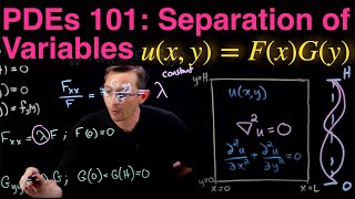
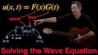
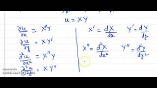
Exactly! We start with u(x, y, t) = X(x)Y(y)T(t). This means we express our solution as a product of functions, each depending on a single variable. Why do we do this?

Because it simplifies the equation into parts we can manage individually?
Correct! By substituting our assumed form into the wave equation, we can isolate different functions related to time and space, making it easier to solve each part independently.
Deriving the Ordinary Differential Equations
🔒 Unlock Audio Lesson
Sign up and enroll to listen to this audio lesson

Let's substitute our assumed solution into the wave equation. Once we do, we can manipulate it to isolate terms involving T, X, and Y. What do we expect to get?

Three separate equations for T, X, and Y?
Exactly! Each part ends up as its own ordinary differential equation. We can represent the temporal part with λ, leading to T'' + λT = 0. This is a classical oscillation equation. What can you tell me about its solutions?

The solutions should be sinusoidal functions, like sine and cosine.
Right again! These solutions represent periodic movement, which is what we want for our membrane.
Normal Modes and Natural Frequencies
🔒 Unlock Audio Lesson
Sign up and enroll to listen to this audio lesson
Finally, as we solve for X(x) and Y(y), we see they take on sine forms. Can anyone explain what 'normal modes' are?
They are patterns of vibration that occur at specific frequencies.
That's correct! Each normal mode corresponds to a unique (n, m) pair, leading to natural frequencies we calculate using ω = √(λ). Can anyone give an example of how these frequencies matter in engineering?
They help us design structures to avoid resonance and vibrations that could be harmful!
Exactly! Understanding these frequencies ensures safety and stability in civil engineering designs.
Introduction & Overview
Read summaries of the section's main ideas at different levels of detail.
Quick Overview
Standard
In this section, the technique of separation of variables is applied to the two-dimensional wave equation. By assuming a product solution and dividing variables, we derive ordinary differential equations that describe the system's behavior. This approach enables the determination of normal modes and natural frequencies of the vibrating membrane.
Detailed
The section focuses on using the method of separation of variables to solve the two-dimensional wave equation that describes the motion of a vibrating membrane. We begin by assuming a solution of the form u(x, y, t) = X(x)Y(y)T(t), where X, Y, and T represent functions dependent on x, y, and t, respectively. Substituting this assumption into the wave equation leads to a separation into three ordinary differential equations (ODEs) upon organizing and dividing.
- The temporal part results in an equation governed by the parameter λ, which describes oscillations over time.
- The spatial components yield equations for X(x) and Y(y), leading to simple harmonic motion solutions like sine functions with boundary conditions defining their behavior at the fixed edges of the membrane.
- The general solution of the system is expressed as a double series of sine functions, multiplied by time-dependent coefficients derived from the initial conditions. This analytical approach allows engineers to characterize normal modes and natural frequencies of membrane vibrations, crucial for applications in civil engineering.
Youtube Videos
Audio Book
Dive deep into the subject with an immersive audiobook experience.
Assumption of the Solution
Chapter 1 of 5
🔒 Unlock Audio Chapter
Sign up and enroll to access the full audio experience
Chapter Content
Assume:
u(x, y,t)=X(x)Y(y)T(t)
Detailed Explanation
In this step, we assume that the solution to the wave equation can be separated into three functions: X(x), Y(y), and T(t). Each function depends on a single variable: X depends only on the position along the x-axis, Y depends only on the position along the y-axis, and T depends only on time t. This assumption simplifies the problem by allowing us to focus on one variable at a time.
Examples & Analogies
Think of a fruit salad where each type of fruit represents a separate function. Just as you can enjoy a strawberry, a banana, or an apple independently while still creating a fruit salad, we can analyze the behavior of each function (X, Y, T) separately to understand the entire solution.
Substituting into the Wave Equation
Chapter 2 of 5
🔒 Unlock Audio Chapter
Sign up and enroll to access the full audio experience
Chapter Content
Substituting into the wave equation:
d2T
(
d2X
d2Y
)
XY =c2 YT +XT
dt2
dx2
dy2
Detailed Explanation
Here, we take the assumption of the solution and substitute it into the two-dimensional wave equation. This gives us an equation that relates the second derivatives of the functions with respect to their respective variables. This substitution is crucial because it transforms the problem into one where we can separate variables.
Examples & Analogies
Imagine a cooking recipe where you need to mix different ingredients. When you substitute the ingredients into your recipe, you start to see how they combine to create a dish. Similarly, substituting the functions into the wave equation allows us to understand how the different parts of our solution interact.
Dividing Both Sides
Chapter 3 of 5
🔒 Unlock Audio Chapter
Sign up and enroll to access the full audio experience
Chapter Content
Dividing both sides by XY T:
1 d2T ( 1 d2X 1 d2Y )
=c2 +
T dt2 X dx2 Y dy2
Detailed Explanation
After substituting into the wave equation, we divide both sides of the equation by the product XYT. This leads to a separation of the equation into distinct parts that can be analyzed separately based on time, position in the x-direction, and position in the y-direction. This is a pivotal step in using the separation of variables technique.
Examples & Analogies
Consider peeling an onion layer by layer. Each layer represents a different variable in our equation. By dividing the equation this way, we effectively peel away the complexity and focus on each individual layer, making it easier to solve.
Defining Lambda and Mu
Chapter 4 of 5
🔒 Unlock Audio Chapter
Sign up and enroll to access the full audio experience
Chapter Content
Let:
1 d2T
=−λ(temporal part)
T dt2
1 d2X 1 d2Y λ
+ =− (spatial part)
X dx2 Y dy2 c2
Split again:
1 d2X 1 d2Y ( λ )
=−μ, =− −μ
X dx2 Y d y2 c2
Detailed Explanation
In this step, we introduce the terms λ and μ. These constants represent spatial and temporal separation in our equation. By setting these equations for T, X, and Y, we create three ordinary differential equations (ODEs) that can each be solved independently. This splitting is fundamental to the separation of variables method.
Examples & Analogies
Imagine you are planning a road trip and need to manage your time and fuel separately. By defining time (λ) for your journey and fuel consumption (μ) as two different concerns, you can optimize your trip more efficiently, just as we optimize our equations by handling each part separately.
Solving Each ODE
Chapter 5 of 5
🔒 Unlock Audio Chapter
Sign up and enroll to access the full audio experience
Chapter Content
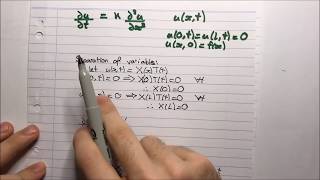
- X″ +μX=0, X(0)=X(a)=0 ⇒ X (x)=sin(nπx/a), μ = (nπ/a)2
- Y″ +νY=0, Y(0)=Y(b)=0 ⇒ Y (y)=sin(mπy/b), ν = (mπ/b)2
- T″ +λT=0, where λ=c2(μ n+ν m) ⇒ T nm(t)=A nmcos(ω nmt)+B nmsin(ω nmt), with ω =√λ=c √(nπ/a)2 + (mπ/b)2
Detailed Explanation
Here we solve the separate ordinary differential equations obtained in the previous step. The solutions involve trigonometric functions (sine), which are suitable for problems with fixed boundaries (like a membrane). Each solution leads to specific terms in the final expression of the displacement function. The constants A and B relate to the initial conditions of motion.
Examples & Analogies
Think of a musician tuning their instrument. Each string must hit the right pitch (like our solved equations). The correct notes produced from these ‘songs’ reflect how well each segment of the equation meets the boundary conditions, ultimately creating a harmonious overall sound from the individual notes.
Key Concepts
-
Separation of Variables: A technique to solve PDEs by breaking down a solution into components dependent on individual variables.
-
Temporal Part: The ODE related to time that emerges after separating variables.
-
Sine Functions: Functions derived from the ODEs characterizing normal modes of vibration in the membrane.
Examples & Applications
Using the separation of variables, the solution for a rectangular membrane can be expressed as a double Fourier sine series, showing how different modes contribute to the overall motion.
The frequencies for the first few modes of a square membrane can be calculated to illustrate their impact on structural design.
Memory Aids
Interactive tools to help you remember key concepts
Rhymes
To find the waves, do it in parts, separated they go, where each one starts.
Stories
Imagine a tightrope walker balancing on a line; the vibrations they make separate into patterns, each with its own time.
Memory Tools
S.I.N.E for understanding: Separation, Isolate, Normalize, Enact!
Acronyms
S.O.V
Separation
Ordinary Equations
Vibrations.
Flash Cards
Glossary
- Separation of Variables
A mathematical method used to solve partial differential equations by expressing them as a product of functions, each depending on a single variable.
- Ordinary Differential Equation (ODE)
A differential equation containing one or more functions of one independent variable and its derivatives.
- Natural Frequencies
Specific frequencies at which a system tends to oscillate in the absence of any driving force.
- Normal Modes
Patterns of motion in a vibrating system that correspond to the system's natural frequencies.
- Boundary Conditions
Constraints applied to the solution of differential equations to reflect physical conditions at the edges of the domain.
Reference links
Supplementary resources to enhance your learning experience.