
Numerical Methods for the 2D Wave Equation
Enroll to start learning
You’ve not yet enrolled in this course. Please enroll for free to listen to audio lessons, classroom podcasts and take practice test.
Interactive Audio Lesson
Listen to a student-teacher conversation explaining the topic in a relatable way.
Introduction to Numerical Methods
🔒 Unlock Audio Lesson
Sign up and enroll to listen to this audio lesson

Today, we’ll learn about why numerical methods are essential when dealing with the two-dimensional wave equation, especially in complex scenarios. Can anyone tell me why we might need these methods?

I think it's because not all problems can be solved using analytical methods?
Exactly! Complex geometries and boundary conditions often make analytical solutions impractical. What are some examples of structures where we might use these numerical methods?

Bridges and building floors?
Correct! Let’s break down two key numerical methods used for these cases.
Finite Difference Method (FDM)
🔒 Unlock Audio Lesson
Sign up and enroll to listen to this audio lesson

Let's discuss the Finite Difference Method. This method involves discretizing our domain into a grid. Who can explain what we mean by that?

Is it about creating a grid of points where we calculate our values?
Yes! We use increments in space (`Δx`, `Δy`) and in time (`Δt`). Following that, we apply a formula to update our values iteratively. Does anyone recall the formula we use?

Is it the one with $u^{n+1}$, $u^n$, and $u^{n-1}$?
Exactly! And we must also consider stability, specifically the CFL condition. Who can explain it briefly?
It ensures the method remains stable over time, right?
Right! Stability is crucial to ensure our numerical solution behaves correctly.
Finite Element Method (FEM)
🔒 Unlock Audio Lesson
Sign up and enroll to listen to this audio lesson
Now, let’s turn to the Finite Element Method, which is powerful for irregular domains. How does FEM differ from FDM?
FEM divides the domain into elements while FDM uses a grid… right?
Spot on! FEM allows for more flexibility in modeling complex shapes. Can someone summarize the steps involved in FEM?
We divide the domain into elements, then approximate the solution using basis functions and finally convert the PDE to algebraic equations using Galerkin's method.
Well done! This versatility makes FEM invaluable in various civil engineering software applications.
Recap and Applications
🔒 Unlock Audio Lesson
Sign up and enroll to listen to this audio lesson
As we wrap up, let’s review the key numerical methods we covered. Who can mention both methods and their key characteristics?
We learned about FDM, which uses a grid, and FEM that works with elements and is more flexible.
Exactly! Can anyone give an example of where we might apply both methods in civil engineering?
For analyzing vibrations in bridges or the structural response of buildings?
Great examples! Numerical methods provide us with the capability to address complex engineering problems effectively.
Introduction & Overview
Read summaries of the section's main ideas at different levels of detail.
Quick Overview
Standard
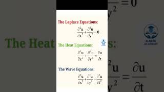
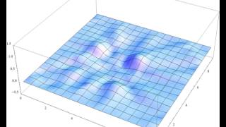
In this section, we explore numerical techniques necessary for solving the complex two-dimensional wave equation, particularly when analytical solutions are not feasible for real-world applications. Key methods discussed are the Finite Difference Method (FDM) and Finite Element Method (FEM), which are critical for modeling membrane behavior under various conditions.
Detailed
Detailed Summary
In civil engineering, solving the two-dimensional wave equation analytically is often infeasible for complex geometries and boundary conditions found in real-world applications. Hence, numerical methods become essential tools for engineers.
Key Numerical Methods
Two commonly used numerical methods discussed in this section include:
1. Finite Difference Method (FDM)
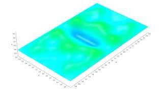
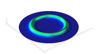
The FDM discretizes the domain into a grid defined by spatial increments (Δx, Δy) and a time increment (Δt). Here, the wave equation is iteratively solved using:
$$ u^{n+1}{i,j} = 2u^{n}{i,j} - u^{n-1}{i,j} + (cΔt)^2 \left(\frac{u{i+1,j} - 2u_{i,j} + u_{i-1,j}}{(Δx)^2} + \frac{u_{i,j+1} - 2u_{i,j} + u_{i,j-1}}{(Δy)^2}\right) $$
The method offers a straightforward approach, but requires adherence to stability criteria, specifically the CFL condition:
$$\frac{(cΔt)^2}{(Δx)(Δy)} \leq 1$$
2. Finite Element Method (FEM)
The FEM is particularly adept at handling irregular domains. It involves:
- Dividing the domain into elements (triangles or quadrilaterals).
- Approximating the solution with basis functions within those elements.
- Applying Galerkin's method to transform the PDE into a solvable system of algebraic equations.
Due to its versatility, FEM is widely employed in professional civil engineering software, enabling accurate modeling of membrane behaviors under loads. This section emphasizes that selecting the appropriate numerical method depends on the complexity of the problem domain and desired solution accuracy.
Youtube Videos


Audio Book
Dive deep into the subject with an immersive audiobook experience.
Introduction to Numerical Solutions
Chapter 1 of 6
🔒 Unlock Audio Chapter
Sign up and enroll to access the full audio experience
Chapter Content
While analytical solutions using separation of variables are useful for simple geometries and boundary conditions, real-world structures often demand numerical solutions due to complexity.
Detailed Explanation
In many cases, the problems we want to solve are too complicated for simple mathematical equations (analytical solutions). This is especially true for real-world structures, which can have complex shapes and varying conditions. Therefore, engineers use numerical methods, which are computational techniques that allow us to approximate these solutions using algorithms instead of exact formulas.
Examples & Analogies
Think of an architect trying to design a modern building. The shapes and loads are often so complex that they cannot be accurately described using traditional mathematics. Instead, they use computer programs that simulate the building’s behavior under various conditions, kind of like a flight simulator for aircraft design.
Finite Difference Method (FDM)
Chapter 2 of 6
🔒 Unlock Audio Chapter
Sign up and enroll to access the full audio experience
Chapter Content
Discretize the domain into a grid:
Let:
- un be the approximation of u(x , y ,t ),
- Δx, Δy: spatial step sizes,
- Δt: time step.
Detailed Explanation
The Finite Difference Method (FDM) involves breaking down a continuous domain (like the surface of a membrane) into smaller, discrete parts called a grid. Each point on this grid represents an approximation of the membrane's displacement at that specific point in time and space. We define step sizes along the axes (Δx for x-direction and Δy for y-direction) as well as a time step (Δt) to determine how often we update the displacement values.
Examples & Analogies
Imagine you are trying to measure the height of a hill not with a tape measure but by using a grid of tiny flags. Each flag represents a measurement point. By measuring the height at each flag position and estimating between them, you can create a complete picture of the hill's shape.
Explicit Finite Difference Scheme
Chapter 3 of 6
🔒 Unlock Audio Chapter
Sign up and enroll to access the full audio experience
Chapter Content
The explicit finite difference scheme for the 2D wave equation is:
un+1 = 2un − un−1 + (cΔt)²
- (un − 2un + un)
- (un − 2un + un)
Detailed Explanation
In this explicit scheme, we update the displacement at the next time step (un+1) based on its current value (un), the value from the previous time step (un−1), and the change due to the nearby points on the grid—affected by the wave speed (c). Essentially, we use the current and past displacements to predict the future displacement, which gives us a way to simulate wave motion over time.
Examples & Analogies
It's like watching a series of waves in a pool. When you throw a stone, you see how the first wave rises (current state), and from that, you predict how the next wave will behave based on the previous ones. You can mentally play out the sequence of waves hitting the edge of the pool, understanding how the water continuously moves.
Stability Criterion (CFL Condition)
Chapter 4 of 6
🔒 Unlock Audio Chapter
Sign up and enroll to access the full audio experience
Chapter Content
Stability Criterion (CFL condition):
(cΔt)²/(Δx Δy) ≤ 1
This ensures that the solution remains stable over time.
Detailed Explanation
The stability criterion, known as the CFL condition, is a critical factor in numerical simulations. It ensures that our predictions do not lead to unrealistic or divergent results over time. By controlling the relationship between the time step (Δt) and the spatial steps (Δx, Δy), we make sure that the method produces stable solutions that behave in a physically meaningful way.
Examples & Analogies
Think about riding a bicycle on a narrow path. If you go too fast (too large of a time step) compared to the width of the path (small space step), you risk falling off the path. Similarly, in numerical simulations, if the time step is too large relative to the spatial resolution, the solution can spiral out of control.
Finite Element Method (FEM)
Chapter 5 of 6
🔒 Unlock Audio Chapter
Sign up and enroll to access the full audio experience
Chapter Content
FEM is more powerful for irregular domains. The basic idea involves:
- Dividing the domain into elements (triangles/quads).
- Approximating the solution using basis functions over each element.
- Applying Galerkin's method to convert the PDE into a system of algebraic equations.
Detailed Explanation
The Finite Element Method (FEM) is particularly useful for modeling more complex geometries that cannot be easily handled by simpler methods. In FEM, the problem domain is divided into smaller, manageable 'elements,' which could be triangular or quadrilateral. Each element has its own approximation based on simple functions (basis functions), and the whole system is assembled to create a larger system of equations that can be solved.
Examples & Analogies
Think of constructing a large puzzle where each piece (element) fits into a complex design. While each puzzle piece is simple, together they create a complete picture. In the same way, FEM breaks down complex problems into smaller parts, allowing for easier solving of the whole.
Application of FEM in Civil Engineering Software
Chapter 6 of 6
🔒 Unlock Audio Chapter
Sign up and enroll to access the full audio experience
Chapter Content
In civil engineering software (e.g., ANSYS, SAP2000), FEM is widely used to model membrane behavior under loads.
Detailed Explanation
Civil engineering software utilizes FEM to analyze how structures (like beams, plates, and membranes) respond to various loads and conditions. By using FEM, engineers can simulate the behavior of materials and structures, evaluate their responses under different loads, and ensure safety and reliability in their designs.
Examples & Analogies
Imagine a game simulation where you can tweak the size and strength of a building model to see how it would react in an earthquake. This kind of modeling allows engineers to design safer buildings by predicting potential failures before actual construction, making it similar to testing a game's effectiveness before launching it.
Key Concepts
-
Numerical Methods: Techniques to solve complex equations when analytical solutions are impractical.
-
Finite Difference Method (FDM): Discretization of space and time for solving wave equations iteratively.
-
CFL Condition: A stability requirement for numerical solutions in wave equations.
-
Finite Element Method (FEM): A method useful for handling irregular domains using piecewise functions.
Examples & Applications
Modeling the vibration of a roof structure using FDM.
Simulating the behavior of a complex bridge under vibrational load using FEM.
Memory Aids
Interactive tools to help you remember key concepts
Rhymes
When the waves travel across the way, use FDM or FEM, that's our play!
Stories
Imagine an engineer faced with a complex bridge design - FDM helps set values in a grid, while FEM allows for flexibility in irregular shapes.
Memory Tools
For stable solutions, remember CFL - Condition for Limitations ensures we don’t derail!
Acronyms
FEM - Flexible Elements Matter; FDM - Fixed Domains Matter.
Flash Cards
Glossary
- Numerical Method
A mathematical approach for solving problems that cannot be solved analytically.
- Finite Difference Method (FDM)
A numerical method for approximating solutions to differential equations by discretizing the domain into a grid.
- CFL Condition
A stability criterion that ensures numerical solutions remain stable over time in the context of wave equations.
- Finite Element Method (FEM)
A powerful numerical technique that divides the domain into smaller elements and approximates solutions using basis functions.
- Galekin’s Method
A method that converts partial differential equations into a system of algebraic equations, widely used in FEM.
Reference links
Supplementary resources to enhance your learning experience.