
Cutoff Frequency Relationship
Enroll to start learning
You’ve not yet enrolled in this course. Please enroll for free to listen to audio lessons, classroom podcasts and take practice test.
Interactive Audio Lesson
Listen to a student-teacher conversation explaining the topic in a relatable way.
Frequency Response Basics
🔒 Unlock Audio Lesson
Sign up and enroll to listen to this audio lesson

Today, we will discuss the frequency response of amplifiers—specifically, common emitter and common source amplifiers. Can anyone tell me why understanding frequency response is important?

I think it helps us know how the gain of the amplifier changes with frequency.
Exactly! As the frequency of the input signal changes, the gain may increase or decrease. We can then analyze this relationship to design better circuits.

What is meant by cutoff frequency?
Good question! The cutoff frequency is where the output power falls to half its maximum value. Remember, this is also the frequency at which our circuit starts behaving differently—the gain levels off or drops!

So, we can say frequencies below the cutoff behave differently compared to those above it?
Yes! Below the cutoff, the circuit will attenuate signals, while above, it will allow them to pass more freely. Let's remember this as the 'cutoff changes gain behavior'—an acronym CGH!
To summarize, understanding frequency response allows us to predict how our amplifier will react to varying input signals, particularly at the cutoff frequency.
Transfer Function Analysis
🔒 Unlock Audio Lesson
Sign up and enroll to listen to this audio lesson

Now let's dive deeper into the transfer function. Who remembers how we derive the transfer function from the circuit's components?

Isn't it done by representing impedances in the Laplace domain and then analyzing the circuit?
Exactly! For a simple RC circuit, we derive the transfer function, noting how the impedance of the capacitor is 1/sC. Can someone help me derive the output-to-input ratio?
We get V(s) = R * I(s) / (R + 1/sC), where I = V(s)/(R + 1/sC). After simplifying, it becomes V(s) = sCR / (1 + sCR).
Well done! This equation illustrates how our gain behaves with frequency. Now, remember that substituting s with jω gives us the frequency response.
So, if we test frequencies, we can find where the gain shifts, right?
Absolutely correct! Understanding these relationships between components is key to mastering circuit analysis.
In summary, we extract the frequency response by analyzing the transfer function and substituting s for jω. This enables us to visualize amplifier behavior.
Behavior of RC Circuits
🔒 Unlock Audio Lesson
Sign up and enroll to listen to this audio lesson
Now, let’s explore how gain varies with frequency in our RC circuit. What do we observe at low frequencies?
Only a minimal amount of signal passes since the capacitor blocks low frequencies.
And, at higher frequencies, the capacitor acts like a short circuit, allowing signals through!
Exactly! At low frequencies, we have significant attenuation; at high frequencies, we allow signals to pass freely! Remember this pattern with the acronym LPHA, for 'Low Pass High Allowance.'
Does this mean that there will be a frequency range where our original signal is effectively unchanged?
Yes! Above the cutoff frequency, the gain stabilizes to a certain value, indicating signal passage. This helps in identifying the pass band of the circuit.
To conclude, our RC circuit demonstrates its behavior as either a filter or a pass-through, depending on the frequency of the applied signal.
Introduction to Bode Plots
🔒 Unlock Audio Lesson
Sign up and enroll to listen to this audio lesson
Next, let’s discuss Bode plots! Why do we use Bode plots instead of linear plots?
Bode plots make it easier to visualize big ranges of frequencies and gains!
Correct! They allow us to effectively represent both gain and phase on a logarithmic scale. When plotting, we consider gains in decibels. Can anyone share the formula for converting to decibels?
It’s 20 times the log of the gain, right?
Absolutely! This helps magnify small signal adjustments across a wide frequency spectrum. Let’s remember the acronym LPGD: 'Logarithmic Plot Gain Decibels!'
And what about the phase part?
The phase will also be plotted on a separate graph against the log frequency. This gives us a complete view of how our circuit behaves at various frequencies.
In summary, Bode plots are beneficial for visualizing gain and phase relationships, providing clarity for circuit analysis across a broad frequency range.
Poles and Cutoff Frequency
🔒 Unlock Audio Lesson
Sign up and enroll to listen to this audio lesson
Now, let's connect what we've learned about transfer functions and poles. Can someone explain what a pole represents?
A pole is a value of s that makes the entire transfer function go to infinity!
Exactly! The pole gives us significant insight into how the system behaves. What about its relationship with cutoff frequency?
So, the cutoff frequency occurs when our transfer function's denominator equals zero, which is the condition for a pole?
Yes! The cutoff frequency derived from the transfer function gives us a crucial understanding of the amplifier's frequency response. Remember: 'Pole-Cutoff Connection'—PCC!
How can we visualize this in terms of frequency response?
By finding where the transfer function denominator zeroes out, we pinpoint our cutoff frequency, where we see a transition change in behavior. It’s vital to grasp this critical relationship!
To summarize, understanding the relationship between poles and cutoff frequency helps us predict circuit behavior in response to varying frequencies.
Introduction & Overview
Read summaries of the section's main ideas at different levels of detail.
Quick Overview
Standard
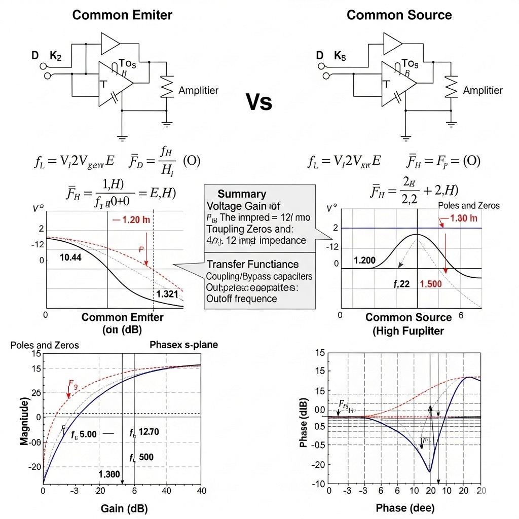
The section delves into the frequency response of common emitter (CE) and common source (CS) amplifiers, emphasizing changes in gain with frequency alterations and exploring the relationship between transfer functions, poles, and cutoff frequencies through RC circuit analysis.
Detailed
In this section, we explore the frequency response of common emitter (CE) and common source (CS) amplifiers, analyzing how the gain varies with the frequency of the input signal. The relationship between the transfer function and frequency response is also examined, particularly the significance of poles and zeros in determining the cutoff frequency. Starting with lower frequency RC circuit analysis, we derive the transfer function and learn to transition from the Laplace domain to the frequency domain by substituting s with jω, thus obtaining the frequency response. We observe that the transfer function behaves as a high-pass filter, displaying unique characteristics at the cutoff frequency, where gain transitions, and phase shifts may occur. Finally, Bode plots are introduced as effective tools for visualizing gain and phase using log scale frequencies, demonstrating their application in practical circuit analysis.
Youtube Videos

Audio Book
Dive deep into the subject with an immersive audiobook experience.
Understanding Cutoff Frequency
Chapter 1 of 4
🔒 Unlock Audio Chapter
Sign up and enroll to access the full audio experience
Chapter Content
So, the corresponding ω; so, this gives us this ω = 1/RC. In fact, what is the significance of this part? It is before this frequency ω we are assuming that 1 was dominating over ωRC magnitude wise and then beyond this point we started saying that you know this part it is now it is going to be dominant.
Detailed Explanation
The cutoff frequency (ω) is a critical point in electrical circuits where the behavior of the circuit changes significantly. It is defined mathematically as 1/(RC), where R is the resistance and C is the capacitance. Below this frequency, the circuit behaves differently compared to above it. The equation shows that when the frequency (ω) is much lower than the cutoff frequency, the term '1' dominates, meaning that the circuit allows signals at low frequencies to pass through easily. However, as the frequency increases and approaches the cutoff frequency, the effects of the RC components become more pronounced, leading to a transition in circuit behavior.
Examples & Analogies
Think of the cutoff frequency like a gate at a park. If you approach the gate slowly (low frequency), it is wide open, and you can pass through easily. However, as you start running (increasing frequency), you have to adjust your speed because soon you'll encounter a point (the cutoff frequency) where the gate starts to close, making it harder to pass. At very high speeds (frequencies) beyond this point, the gate becomes fully closed, and you can no longer enter.
Dominance of Impedance Terms
Chapter 2 of 4
🔒 Unlock Audio Chapter
Sign up and enroll to access the full audio experience
Chapter Content
At the frequency where ω = ω1, both the jωRC part and the constant part balance out. Therefore, one can approximate the transfer function based on which term is dominating, whether it's the capacitive reactance (jωRC) or the resistance (R).
Detailed Explanation
This chunk discusses how the circuit's transfer function is influenced by the relative dominance of the capacitive reactance (represented by jωRC) or the resistance (R) at various frequencies. At the cutoff frequency (ω1), the two terms are equal; this is significant because it marks the transition point of circuit behavior. Below ω1, the impedance of the resistor dominates, while above ω1, the capacitive reactance starts to dominate. This understanding allows us to make approximations about the circuit's behavior, simplifying analysis.
Examples & Analogies
Imagine a see-saw balanced perfectly in the middle: that's like the cutoff frequency where both forces (the jωRC and R) balance out. When one side (force) becomes stronger, like when kids sit on one side of the see-saw, it tips to one side—this represents how the circuit reacts differently to high or low frequencies.
Magnitude Response and Phase Shift
Chapter 3 of 4
🔒 Unlock Audio Chapter
Sign up and enroll to access the full audio experience
Chapter Content
As we consider the frequency response, the magnitude (gain) of the output compared to the input signal changes with frequency. At low frequencies, the gain is low, and as frequency increases, the gain approaches 1. Also, phase shift occurs, moving from 90° to 0° across the cutoff frequency.
Detailed Explanation
The magnitude response details how much of the input signal is available at the output as the frequency varies. Initially, at lower frequencies, the gain is low due to the dominance of the capacitor. However, as the frequency increases, the output approaches the input level, resulting in a gain of 1 (or 0 dB). Simultaneously, the phase shift begins at 90° (indicating a delay in response) and decreases to 0° as frequency further increases. This means the output signal is less delayed and starts to closely follow the input.
Examples & Analogies
Consider a runner (the output signal) racing against a train (the input signal). At slow speeds (low frequencies), the runner struggles to keep up, so they lag behind (low gain). As both increase speed (frequency rises), the runner becomes synchronized with the train, reaching a point where they run side by side (gain reaches 1). At very high speeds, the runner keeps up perfectly, and there’s no delay in the response (phase shift becomes 0°).
Cutoff Frequency and Transfer Function Relationship
Chapter 4 of 4
🔒 Unlock Audio Chapter
Sign up and enroll to access the full audio experience
Chapter Content
This cutoff frequency is directly related to the poles in the transfer function of the system in the Laplace domain, where the transfer function becomes infinite.
Detailed Explanation
The cutoff frequency discussed earlier has a significant relationship with the concept of poles in control systems. A pole in the transfer function at s=0 means that at this point, the transfer function approaches infinity, indicating a frequency where the system can no longer respond linearly to input signals. Understanding this relationship helps in designing systems that act predictively within desired frequency ranges.
Examples & Analogies
Imagine a crowded concert where the sound quality varies. If too many people (poles) try to enter the concert together, it becomes overwhelming, and the music sounds distorted (infinite response). At a certain point (cutoff frequency), the entrance can handle the crowd dynamically, allowing for a balance in sound quality and flow as the audience moves in and out (frequency response becomes manageable).
Key Concepts
-
Frequency Response: The way gain varies with input frequency, important for understanding circuit performance.
-
Cutoff Frequency: A critical point that indicates transition from pass to stop band behavior in amplifiers.
-
Transfer Function: A mathematical model used to understand input-output relationships in circuits.
-
Poles and Zeros: Points in the transfer function that define system behavior and frequency response characteristics.
Examples & Applications
An RC high-pass filter exhibits an increase in gain with increasing frequency but significantly attenuates signals below a certain cutoff frequency.
In a common emitter amplifier, the frequency response can demonstrate significant phase shifts and gain variations, making it crucial to consider the input signal frequency.
Memory Aids
Interactive tools to help you remember key concepts
Rhymes
In circuits we find a cutoff line, where signals mute and gain declines.
Stories
Imagine a racing car accelerating through narrow winding roads; initially slow, but as it reaches a certain speed, it finds more freedom, much like gain increasing above the cutoff frequency.
Memory Tools
Remember ‘POLAR’ for Poles, Output, Lag, Amplification, and Response relating to transfer functions and frequency analysis.
Acronyms
Use ‘CRF’ to remember Cutoff Frequency, Response, Filter for easy recall of key components!
Flash Cards
Glossary
- Cutoff Frequency
The frequency at which the output power of a circuit falls to half its maximum value, marking a transition point in amplifier behavior.
- Transfer Function
A mathematical representation that describes the relationship between the input and output of a system in the Laplace domain.
- Pole
A value of the complex variable 's' in the transfer function that causes the function to approach infinity, indicating a critical point in circuit response.
- Frequency Response
The behavior of an amplifier or circuit's gain as a function of frequency.
- Bode Plot
A graphical representation of the gain and phase of a system plotted against logarithmic frequency, commonly used in control theory.
Reference links
Supplementary resources to enhance your learning experience.