
Numerical Example: 2-DOF System
Enroll to start learning
You’ve not yet enrolled in this course. Please enroll for free to listen to audio lessons, classroom podcasts and take practice test.
Interactive Audio Lesson
Listen to a student-teacher conversation explaining the topic in a relatable way.
Understanding Mass and Stiffness Matrices
🔒 Unlock Audio Lesson
Sign up and enroll to listen to this audio lesson

Today, we’ll start by discussing the mass and stiffness matrices for a 2-DOF system. These matrices play a crucial role in understanding how the system behaves under dynamic loads.

Can you explain what the mass matrix is exactly?
Absolutely! The mass matrix reflects the distribution of mass in the system. In our example, it looks like this: [M] = [[m1, 0], [0, m2]]. Each diagonal element represents the mass at each degree of freedom.

What about the stiffness matrix? How is that formed?
Great question! The stiffness matrix defines how hard it is for the structure to deform. Our stiffness matrix is [K] = [[k1 + k2, -k2], [-k2, k2]]. The off-diagonal terms reflect interaction between degrees of freedom.

Nice! I see how both matrices contribute to the system’s response.
Exactly! And understanding them is vital for the next steps in our analysis. Now let's move on to calculating natural frequencies.
Calculating Natural Frequencies and Mode Shapes
🔒 Unlock Audio Lesson
Sign up and enroll to listen to this audio lesson

Once we have our mass and stiffness matrices, we can calculate natural frequencies. This involves solving the eigenvalue problem: [K] - ω²[M] = 0.

What do ω² represent in this context?
ω² are the eigenvalues, which represent the natural frequencies squared. The corresponding eigenvectors will give us the mode shapes.
Can you provide an example of what one of those calculations looks like?
Sure, once we solve the characteristic equation, we can find the values of ω and also determine the modal response. The mode shapes will tell us how each part of the structure moves relative to the others.
Sounds complex but interesting! Does it apply directly to seismic analysis?
Absolutely! Knowing the natural frequencies and mode shapes is key to evaluating how a structure will respond to ground motion.
Response to Ground Motion
🔒 Unlock Audio Lesson
Sign up and enroll to listen to this audio lesson
Now let’s talk about how to estimate the system's response to ground motion once we have natural frequencies and mode shapes.
What are the two methods we can use for this?
We can apply either modal superposition or the response spectrum method. Modal superposition breaks down the response into contributions from each mode.
What about the response spectrum method? What makes it different?
The response spectrum method uses a graph derived from recorded ground motions to estimate maximum responses for each mode. It’s a powerful way to analyze seismic forces efficiently.
That sounds really useful for practical applications!
Indeed! Remember, understanding these concepts is essential for realistic dynamic analyses in structural engineering. Let’s recap: we discussed mass and stiffness matrices, calculated natural frequencies, and explored how to respond to ground motion.
Introduction & Overview
Read summaries of the section's main ideas at different levels of detail.
Quick Overview
Standard
The section outlines the process of establishing the mass and stiffness matrices for a 2-DOF system. It provides the framework for calculating natural frequencies, mode shapes, and the system's response to ground motion through modal superposition or response spectrum methods.
Detailed
Numerical Example: 2-DOF System
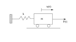
This section focuses on a typical worked-out numerical example involving a 2-degree-of-freedom (2-DOF) system crucial for understanding the dynamic response of such systems in structural analysis. The example begins with defining the mass and stiffness matrices:
- Mass matrix and Stiffness matrix for a simplified 2-DOF system are given as:
$$
[M] = \begin{bmatrix}
\ m_1 & 0 \
0 & m_2
\end{bmatrix}
$$
$$
[K] = \begin{bmatrix}
k_1 + k_2 & -k_2 \
-k_2 & k_2
\end{bmatrix}
$$
The section illustrates how to solve for crucial dynamic characteristicsincluding:
- Natural frequencies: Solutions for the natural frequencies of the 2-DOF system derived from the eigenvalue problem.
- Mode shapes: Calculation of corresponding mode shapes (eigenvectors) associated with each natural frequency.
- Modal participation: The contribution of each mode to the overall dynamic response.
- Response to ground motion: Application of modal superposition or the response spectrum method to estimate the system's response under seismic loading.
This numerical example reinforces the theoretical concepts discussed earlier in the chapter, proving essential for practical applications in dynamic analysis.
Youtube Videos

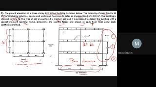
![Numerical from past question on basic structural dynamics||Earthquake Engineering|| [Lec-2]](https://img.youtube.com/vi/36ApBVBLxhA/mqdefault.jpg)


Audio Book
Dive deep into the subject with an immersive audiobook experience.
Mass Matrix Definition
Chapter 1 of 3
🔒 Unlock Audio Chapter
Sign up and enroll to access the full audio experience
Chapter Content
Mass matrix:
\[ [M] = \begin{bmatrix} m_1 & 0 \ 0 & m_2 \end{bmatrix} \]
Where \( m_1 \) and \( m_2 \) are the masses at the two degrees of freedom.
Detailed Explanation
The mass matrix represents the masses associated with each degree of freedom in a two-degree-of-freedom (2-DOF) system. Each entry of the diagonal matrix corresponds to the mass at a specific point in the system. For instance, \( m_1 \) is the mass at the first DOF and \( m_2 \) is the mass at the second DOF, while off-diagonal entries are zero, indicating that there isn't mass coupling between the two DOFs.
Examples & Analogies
Imagine you have two identical swinging pendulums attached at different heights; each pendulum's mass can be thought of as a point on a scale. The mass matrix tells you how heavy each pendulum is at its swinging point, irrespective of how they influence each other.
Stiffness Matrix Definition
Chapter 2 of 3
🔒 Unlock Audio Chapter
Sign up and enroll to access the full audio experience
Chapter Content
Stiffness matrix:
\[ [K] = \begin{bmatrix} k_1 + k_2 & -k_2 \ -k_2 & k_2 \end{bmatrix} \]
Where \( k_1 \) and \( k_2 \) are the stiffness constants of the system.
Detailed Explanation
The stiffness matrix defines how both degrees of freedom resist deformation when forces are applied. The diagonal entries represent the total stiffness associated with each DOF, and the off-diagonal entries show how the stiffness of one DOF affects the other DOF. For example, \( k_1 \) and \( k_2 \) could represent stiffness from springs connected to each mass, where the negative off-diagonal terms indicate interactions between the two masses.
Examples & Analogies
Think of two springs connected to each other. When one spring is compressed, it not only pushes back against its own deformation but also affects the other spring. The stiffness matrix is like a recipe that tells you how these springs will work together to resist forces.
Solving for Natural Frequencies
Chapter 3 of 3
🔒 Unlock Audio Chapter
Sign up and enroll to access the full audio experience
Chapter Content
Solving for:
- Natural frequencies
- Mode shapes
- Modal participation
- Response to ground motion (using modal superposition or response spectrum)
Detailed Explanation
To analyze a 2-DOF system, engineers calculate the natural frequencies, which are the frequencies at which the system tends to oscillate when disturbed. The modal shapes describe how each mass moves during these oscillations. This analysis helps predict how the system will respond during events like earthquakes. Modal participation factors can be used to understand how effective each mode is in contributing to overall motion, and finally, the response to ground motions is calculated using modal superposition, which combines the effect of the oscillation modes to get a complete picture.
Examples & Analogies
Imagine a swing (the natural frequency) at a playground where children play. If one child swings at their frequency, they create a different motion compared to when the swing is empty. Each child's unique way of swinging represents different modes of vibration. By analyzing how they swing together, you can foresee how the swings will behave when someone starts pushing them (like ground motion during an earthquake).
Key Concepts
-
Mass Matrix: A representation of the distribution of mass across the DOFs in a system.
-
Stiffness Matrix: A representation of the stiffness of the system defined by its components.
-
Natural Frequencies: Frequencies at which the system can oscillate without external forces.
-
Mode Shapes: The patterns of motion corresponding to each natural frequency in the system.
-
Modal Analysis: A technique used to study the dynamic response of systems.
Examples & Applications
For a 2-DOF system with mass values m1=10 kg and m2=20 kg, the mass matrix would be [M] = [[10, 0], [0, 20]].
If the stiffness constants are k1=15 N/m and k2=5 N/m, the stiffness matrix becomes [K] = [[20, -5], [-5, 5]].
Memory Aids
Interactive tools to help you remember key concepts
Rhymes
In two masses we trust, their motion is a must; Stiffness shows the way, to keep vibrations at bay.
Stories
Imagine two friends on a seesaw. They bounce up and down, representing the natural frequencies and mode shapes in our 2-DOF system having fun while balancing.
Memory Tools
M for Mass, S for Stiffness, N for Natural Frequencies: M, S, N helps remember the sequence of key components.
Acronyms
MNS - Remember
Mass
Natural Frequency
and Stiffness as the critical components in dynamic analysis.
Flash Cards
Glossary
- Degree of Freedom (DOF)
An independent displacement or rotation needed to define the configuration of a structure.
- Mass Matrix
A matrix representing the distribution of mass in a system, essential for dynamic analysis.
- Stiffness Matrix
A matrix that defines how resistant a structure is to deformation under load.
- Natural Frequency
The frequency at which a system tends to oscillate in the absence of any driving force.
- Mode Shapes
The shapes that a structure assumes at its natural frequencies during vibration.
- Modal Superposition
A technique where the response of a multi-degree-of-freedom system is simplified to the sum of responses from individual modes.
- Response Spectrum
A graph that represents the peak response of a structure to various frequencies of ground motion.
Reference links
Supplementary resources to enhance your learning experience.