
Numerical Solution Methods for MDOF Systems
Enroll to start learning
You’ve not yet enrolled in this course. Please enroll for free to listen to audio lessons, classroom podcasts and take practice test.
Interactive Audio Lesson
Listen to a student-teacher conversation explaining the topic in a relatable way.
Overview of Numerical Methods
🔒 Unlock Audio Lesson
Sign up and enroll to listen to this audio lesson

Today, we'll explore the numerical solution methods for MDOF systems. Why do you think analytical methods are not always feasible for these systems?

I think because MDOF systems are more complex than SDOF systems?
Exactly! As we increase the number of degrees of freedom, the equations become more complex, making analytical solutions less practical. Hence, we rely on numerical integration methods. What are some examples of these methods?

Is the Newmark-beta Method one of them?
Yes! The Newmark-beta method is indeed one of the key techniques used. It's known for its unconditional stability under specific conditions. Let's explore some more methods.
Deep Dive into Time Integration Methods
🔒 Unlock Audio Lesson
Sign up and enroll to listen to this audio lesson

Now, let's gain insights into the time integration methods. Who can summarize the characteristics of the Wilson-θ method?

The Wilson-θ method is stable for larger time steps, right?
Correct! Stability with larger time steps is crucial for accurately modeling dynamic responses. Does anyone know about Runge-Kutta methods?

I believe they are explicit methods that maintain conditional stability?
Right on! They are popular in various engineering analyses due to their versatility.
Introduced Concepts of Modal Truncation
🔒 Unlock Audio Lesson
Sign up and enroll to listen to this audio lesson
Now that we've gone through the integration methods, let's discuss modal truncation. Why do you think truncating the modes is beneficial?
It helps reduce the computational workload, right?
Absolutely! Focusing on just the first few dominant modes simplifies our analysis while still accurately reflecting the system's behavior under seismic loads. How many modes do we usually consider?
I think it’s usually the first 3 to 5 modes.
Exactly! Well done! By truncating our modal analysis to these primary modes, we can efficiently conduct our dynamic analyses.
Introduction & Overview
Read summaries of the section's main ideas at different levels of detail.
Quick Overview
Standard
Numerical solution methods are necessary for analyzing MDOF systems due to the infeasibility of analytical solutions for larger structures. The section highlights various time integration methods and the concept of modal truncation to enhance computational efficiency.
Detailed
Numerical Solution Methods for MDOF Systems
In the analysis of Multi-Degree-of-Freedom (MDOF) systems, analytical solutions become impractical as the complexity of the structures increases. Thus, numerical integration methods are utilized, particularly for large-scale problems often encountered in real-world structures.
16.8.1 Time Integration Methods
Various time integration techniques are available to analyze dynamic systems:
- Newmark-beta Method: A widely used method known for its unconditional stability under certain parameters.
- Wilson-θ Method: Ensures stability for larger time steps, making it suitable for specific analysis needs.
- Runge-Kutta Methods: Explicit methods that offer conditional stability, effective in different analytical scenarios.
These techniques allow us to simulate the dynamic response of MDOF systems under various loading conditions effectively.
16.8.2 Modal Truncation
In dynamic analysis, it is noted that only a few dominant modes (typically the first 3–5) significantly influence the structure's response during seismic loading. This realization helps in reducing the computational effort required for solving MDOF systems, allowing for efficient and practical analysis while maintaining accuracy.
Youtube Videos


Audio Book
Dive deep into the subject with an immersive audiobook experience.
Introduction to Numerical Solutions
Chapter 1 of 3
🔒 Unlock Audio Chapter
Sign up and enroll to access the full audio experience
Chapter Content
Analytical solutions are feasible only for small systems. For real structures, numerical integration is essential.
Detailed Explanation
Analytical solutions refer to mathematical solutions derived using direct calculations. These solutions work well for small-scale problems but become impractical for larger, more complex systems like real-world structures. Consequently, engineers use numerical integration methods to approximate solutions for these larger structures. Numerical methods break down complex equations into simpler, more workable problems that can be solved using computers.
Examples & Analogies
Think of analytical solutions like trying to solve a simple equation by hand, such as 2 + 2 = 4. But when you have to deal with a complicated problem, like predicting the course of a hurricane or managing the traffic flow in a city, it becomes complex, and manual calculations won’t suffice. Instead, we rely on computers to crunch many numbers simultaneously and give us results that are good enough to make decisions.
Time Integration Methods
Chapter 2 of 3
🔒 Unlock Audio Chapter
Sign up and enroll to access the full audio experience
Chapter Content
16.8.1 Time Integration Methods
• Newmark-beta Method: Widely used, unconditionally stable for certain parameters.
• Wilson-θ Method: Stable for large time steps.
• Runge-Kutta Methods: Explicit, conditionally stable.
Detailed Explanation
When it comes to analyzing dynamic systems, we need to understand how these systems behave over time. Time integration methods help engineers simulate the response of MDOF systems to different loading conditions over time.
- Newmark-beta Method is popular due to its stability under certain conditions. It allows engineers to accurately predict how structures behave during events such as earthquakes.
- Wilson-θ Method is advantageous when time steps are larger, providing stability in predictions even when calculations are spread over longer periods.
- Runge-Kutta Methods are a family of methods that give accurate results for many problems but can impose restrictions on the size of the time step to maintain accuracy.
Examples & Analogies
Consider a car traveling down a curvy road. If you want to predict how your car will move, you might need to take measurements at various points along the way to understand the trajectory. Time integration methods are like taking those measurements at regular intervals. If the road is simple and straight (like a small system), you can calculate the route by hand. But if the road is complicated (like real structures), you need a robust technique to simulate how the car might move at different times, ensuring safety and efficiency.
Modal Truncation
Chapter 3 of 3
🔒 Unlock Audio Chapter
Sign up and enroll to access the full audio experience
Chapter Content
16.8.2 Modal Truncation
Only a few dominant modes (typically the first 3–5) contribute significantly to dynamic response, especially for seismic analysis. This helps reduce computational effort.
Detailed Explanation
In analyzing MDOF systems, especially during dynamic events like earthquakes, not all modes are equally important. Research shows that generally, just a small number of modes—typically the first three to five—have a substantial influence on the system's overall response. By focusing on these key modes, engineers can simplify calculations, making the analysis faster and less resource-intensive while still achieving reliable results.
Examples & Analogies
Imagine you are listening to your favorite song. There are multiple instruments playing, but the vocals and a prominent guitar solo are what you notice the most. If you were to analyze the song, you could focus only on those key parts rather than trying to account for every single note from every instrument. This analogy of focusing on the dominant sounds in music can help us understand how modal truncation works—by simplifying the complex MDOF system into its most influential components for efficient analysis.
Key Concepts
-
Numerical Integration: Computational techniques for solving differential equations.
-
Time Integration Methods: Approaches to approximate solutions for time-dependent systems.
-
Modal Truncation: Simplifying dynamic analysis by focusing on dominant modes.
Examples & Applications
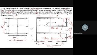
Using the Newmark-beta method to analyze seismic response in a multi-storey building.
Employing modal truncation to focus on the first three modes of an MDOF system to simplify computational efforts.
Memory Aids
Interactive tools to help you remember key concepts
Rhymes
In MDOF systems, we take our bets, with numerical methods, no regrets.
Stories
Imagine engineers at a big construction site. They realized that trying to solve every mode's response analytically was a daunting task. They found a treasure map of numerical methods leading them to quicker solutions! And with modal truncation, they learned to ignore the noise of excessive calculations.
Memory Tools
To remember time integration methods: NWR - Newmark, Wilson, Runge-Kutta.
Acronyms
TIME - Truncate Integrate Modes Efficiently.
Flash Cards
Glossary
- Numerical Integration
A range of computational methods used to solve differential equations numerically, often applied in dynamic analysis.
- Time Integration Methods
Specific techniques used to approximate the solutions of dynamic equations over time, key for analyzing systems subjected to time-varying loads.
- Modal Truncation
The practice of considering only a few significant modes in a dynamic analysis to reduce computational effort while maintaining accuracy.
Reference links
Supplementary resources to enhance your learning experience.