
Velocity Field Estimation
Enroll to start learning
You’ve not yet enrolled in this course. Please enroll for free to listen to audio lessons, classroom podcasts and take practice test.
Interactive Audio Lesson
Listen to a student-teacher conversation explaining the topic in a relatable way.
Introduction to Velocity Fields
🔒 Unlock Audio Lesson
Sign up and enroll to listen to this audio lesson

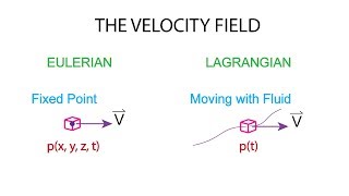
Today, we're diving into velocity fields! This involves using Navier-Stokes equations. First up, can anyone explain what we mean by a velocity field in fluid mechanics?

Is that how we describe the speed and direction of fluid flow?
Exactly! We can quantify this velocity field due to pressure gradients. For example, when we have parallel plates, we derive it as u = -dp/dx multiplied by some fluid variables. Can someone tell me why we might neglect gravity?

If gravity is negligible, it simplifies the calculations, right?
Right! This allows us to focus on shear stress and vorticity that are more influential under certain conditions. Remember: gravity complications can obscure specific insights.

What's vorticity again? I think it's related to rotation!
Yes! Vorticity is a measure of rotation in the fluid. We'll calculate it from the flow velocities too. Keep this in mind, as it plays a role in distinguishing irrotational from rotational flows.

So, what would one do if potential functions don't exist?
Good question! We focus on average velocity calculations when the flows aren’t irrotational. Hence, the concept of boundary layers becomes significant in forecasting real-world behaviors.
In summary, we grasp how velocity fields form through both static equations and dynamic implications. Remember to relate pressure and shear when thinking of fluid flows.
Wall Shear Stress Calculations
🔒 Unlock Audio Lesson
Sign up and enroll to listen to this audio lesson

We’re going deeper now—let's discuss calculating wall shear stress. Can anyone remind me what Newton's law of viscosity states?
It suggests that shear stress is directly proportional to the rate of strain in the fluid.
Correct! So at the wall, we can just apply this to derive tau_xy = mu * (du/dy). Why is this important?
It helps us understand how much stress is on the walls due to fluid motion.
Exactly! The stress at walls impacts design and material choices in engineering. Can anyone calculate tau_xy if we have a max velocity u_max at the wall?
Wouldn’t it be tau = 2mu * u_max?
Spot on! Understanding shear stress distributions is crucial when designing systems subjected to these conditions.
So, remember that wall shear stresses dictate flow behavior near surfaces and reflect upon your material science applications!
Stream Functions and Their Importance
🔒 Unlock Audio Lesson
Sign up and enroll to listen to this audio lesson
Let’s now tackle stream functions. Who can explain how we define stream functions in flow?
Isn’t it related to the continuity equation for the flow?
Exactly! In two-dimensional flow, a stream function helps visualize flow patterns. We integrate velocities to find it. What do we do with the value of psi at the center line?
We set it to zero as a reference point!
Right! That gives us a baseline from where we can measure other values. It’s essential in determining flow direction and volume. Why is knowing boundaries significant?
It tells us about the regions where flow is critical, especially near surfaces!
Exactly! Always consider the implications of fluid behavior around boundaries when discussing practical applications.
In summary, stream functions greatly enhance our understanding of flow dynamics. Always tie these concepts back to flow visualization!
Velocity Potential Limitations
🔒 Unlock Audio Lesson
Sign up and enroll to listen to this audio lesson
Now, let’s think critically—what’s our understanding of velocity potentials? When can we use them?
They can be used in irrotational flows, right?
Exactly! In flows with vorticity, the potential functions can’t be established. Why is understanding this important in applications?
It could influence how we analyze flow systems since we might be misled without proper definitions.
Well put! Always ensure to check for vorticity presence before attempting potential calculations in practical scenarios.
In conclusion, recognizing the limits of potential functions aids all of our problem-solving approaches in fluid dynamics!
Application of Average Velocity Calculations
🔒 Unlock Audio Lesson
Sign up and enroll to listen to this audio lesson
To finish our series, let’s discuss average velocity. How do we arrive at average velocity in a system?
I think it relates to integrating velocity across an area, right?
Correct! Average velocity can be computed through integration over area dictated by your flow configuration. Why is this important?
It helps illustrate average flow characteristics that can dictate design choices.
Precisely! Adequately approximating these characteristics allows for more effective system designs in engineering applications. What could a high average velocity indicate?
It could signal higher kinetic energy in the system, requiring careful handling in designs.
Right again! Always evaluate average velocity in relation to your system or design implications. Very well done, everyone!
Introduction & Overview
Read summaries of the section's main ideas at different levels of detail.
Quick Overview
Standard
The section outlines how to estimate velocity fields using Navier-Stokes equations, explores shear stress and vorticity, and elaborates on stream functions and velocity potential in a two-dimensional flow. It emphasizes fluid behavior under various conditions and the importance of understanding boundary layers for practical applications.
Detailed
Velocity Field Estimation
This section provides an in-depth exploration of how fluid velocity fields can be estimated, particularly using the Navier-Stokes equations. The section begins with the basic definitions of fluid mechanics concepts such as wall stress, shear stress, stream function, vorticity, velocity potential, and average velocity. The reader learns how to derive these properties by substituting into Navier-Stokes equations under the assumption of zero gravitational force and considering constant pressure gradient conditions.
Key Points
- Velocity Field Calculation: The velocity field of a fluid can be expressed as a function of the pressure gradient
$$
u = -\frac{dp}{dx} \cdot \frac{h^2}{2\mu}(1 - \frac{y^2}{h^2})
$$
Here, h is the half-gap between two parallel plates, and µ is the dynamic viscosity. This suggests that velocity gradient conditions define how fluid moves between boundaries.
-
Wall Shear Stress: Discussing how to use Newton's laws of viscosity to compute the wall shear stress,
$$\tau_{xy} = \mu \cdot \frac{du}{dy}$$ is key to understanding fluid mechanics around boundaries. The application of derivatives aids in deriving relevant values at defined points in the flow. - Stream Function and Vorticity: In two-dimensional flow, the stream function can be integrated from the velocity definitions, which leads us to consider the flow direction and the dynamics of rotational and irrotational flow. Vorticity is investigated by taking curls and determining field characteristics.
- Velocity Potential: An important determinant in fluid dynamics, however, it is confirmed that potential function does not exist in rotational flows effectively eliminating certain considerations.
- Average Velocity Calculation: Finally, for practical use cases like tank flows, the average velocity can be defined through a discharge formulation leading to the understanding of flow characteristics.
The section wraps up by contemplating simplifications used in computational fluid dynamic approaches, highlighting the vital understanding of boundary layer approximations – critical for real-life applications.
Youtube Videos
![Introduction to Velocity Fields [Fluid Mechanics #1]](https://img.youtube.com/vi/CkNo5xGMZS4/mqdefault.jpg)


Audio Book
Dive deep into the subject with an immersive audiobook experience.
Overview of Velocity Field
Chapter 1 of 5
🔒 Unlock Audio Chapter
Sign up and enroll to access the full audio experience
Chapter Content
This section discusses how to estimate the wall stress, shear stress, stream function, vorticity, velocity potential, and average velocity using the previously solved velocity field based on the Navier-Stokes equations.
Detailed Explanation
In fluid mechanics, when estimating the velocity field, we look at various parameters like wall stress and shear stress. The velocity field gives us insight into how the fluid moves and behaves when subjected to forces. In our previous classes, we derived this velocity field using the Navier-Stokes equations, which are fundamental equations governing fluid motion. We made simplifying assumptions like neglecting gravity and assuming certain boundary conditions (like the fluid’s velocity at the wall being zero). These equations allow us to analyze and calculate not just the velocity but also related aspects such as shear stress and vorticity.
Examples & Analogies
Think about how water flows out of a tap. When you turn the tap on, the water’s velocity starts low and increases as it flows out. Understanding the velocity field is akin to determining how fast and in what manner the water flows as it exits the tap. The moment you start calculating things like the speed at different points or how pressure changes within the water stream, you are applying concepts similar to those in the derivation of velocity fields in fluid mechanics.
Wall Shear Stress Calculation
Chapter 2 of 5
🔒 Unlock Audio Chapter
Sign up and enroll to access the full audio experience
Chapter Content
Using Newton's laws of viscosity, we can substitute to find the wall shear stress (tau_xy) using the equation that relates it to the changes in velocity at the wall.
Detailed Explanation
Wall shear stress is a critical parameter in fluid mechanics that quantifies the tangential force per unit area at the boundary of a fluid flow. To calculate this, we apply Newton’s law of viscosity, which states that the shear stress is proportional to the velocity gradient. By taking partial derivatives of our velocity field, we can determine how the fluid speed changes near the wall (where y equals ±h). These calculations lead us to express the shear stress in terms of the pressure gradient and fluid properties. The final calculated shear stress is fundamental for understanding how forces are transmitted in a fluid near the boundary.
Examples & Analogies
Consider a swimmer pushing against the water as they try to move forward. The water near their hands experiences shear stress due to their movement and pushes against them. By understanding how the speed of water changes near their hands (the wall), they can estimate how much effort (force) they need to exert - similar to calculating wall shear stress in fluid flow.
Stream Functions in Two-Dimensional Flow
Chapter 3 of 5
🔒 Unlock Audio Chapter
Sign up and enroll to access the full audio experience
Chapter Content
For a two-dimensional steady incompressible flow, we can derive stream functions by integrating the velocity fields, setting the stream function value to zero at the center line.
Detailed Explanation
Stream functions are used in fluid mechanics to represent flow patterns in two-dimensional flows. By integrating the velocity field, we can generate a mathematical function that describes how streamlines behave. By setting the function's value to zero at a central line, we establish reference points that help visualize and calculate the streamlines - which are paths followed by fluid particles. Each streamline is analogous to the trail left by a moving object and helps in understanding how fluid behaves under certain conditions.
Examples & Analogies
Imagine a crowded room where people are moving to exit through a doorway. The paths that people take can be likened to streamlines. If we were to track the trajectories of individuals, we could map them out much like stream functions in fluid flow, showing how efficiently the room empties, akin to analyzing how smoothly a fluid flows through a pipe.
Understanding Vorticity
Chapter 4 of 5
🔒 Unlock Audio Chapter
Sign up and enroll to access the full audio experience
Chapter Content
Vorticity in the zth plane relates to how the fluid rotates or circulates about a point in the plane. We derive this from the fluid's velocity field.
Detailed Explanation
Vorticity measures the local rotational motion of a fluid and is defined mathematically via the curl of the velocity field. In simple terms, when a fluid moves, it may twist and turn rather than just move in a straight line. Vorticity provides a quantifiable way to analyze how and where such rotations are happening within a fluid. This is essential for understanding complex flow behaviors and interactions between different velocity fields, such as those found in turbulent flows.
Examples & Analogies
Think of a small whirlpool that forms when water drains in a bathtub. The water swirls around a central point, creating rotational motion. This swirling motion is a representation of vorticity. Understanding this concept helps us identify how fluids behave in various situations, from small-scale whirlpools to large ocean currents.
Average Velocity Calculation
Chapter 5 of 5
🔒 Unlock Audio Chapter
Sign up and enroll to access the full audio experience
Chapter Content
We calculate the average velocity through integrating the product of the velocity and the differential area over the flow region, then dividing by the total area.
Detailed Explanation
Average velocity is calculated using an integration approach where the total velocity (multiplied by differential area elements) is summed across the entire flow region divided by the total area. This provides a representative value of the velocity at which fluid flows through a given cross-section. It's a crucial calculation in fluid dynamics, as it impacts how we design systems such as pipes or channels that carry fluids.
Examples & Analogies
Consider a river flowing with varying speeds at different points across its width. If you wanted to know the average speed of the river, you could measure speeds at small sections, calculate the contribution of each section based on its area, and combine them to find an overall average. This helps us understand flow rates and how to manage water resources efficiently.
Key Concepts
-
Velocity Field: Represents how fluid velocities are distributed across space.
-
Shear Stress: Key to understanding the interaction between fluids and solid surfaces.
-
Vorticity: Important for analyzing rotational flow behavior.
-
Stream Function: Aids in visualizing flow patterns and characteristics.
-
Velocity Potential: Exists only in irrotational flows; essential in defining flow behaviors.
-
Average Velocity: A valuable metric that helps evaluate flow systems.
Examples & Applications
In a pipe flow, if the pressure gradient is large, the velocity field will show a significant increase in fluid speed as it approaches the exit.
When estimating the shear stress on the walls of a tank being filled, we could apply Navier-Stokes to find how pressures change with respect to flow speed.
Memory Aids
Interactive tools to help you remember key concepts
Rhymes
In fluid flow, listen here, velocity fields will appear, with shear stress and vorticity, make your understanding clarity!
Stories
Imagine a river flowing between two banks; as the water speeds up, the pressure changes and the fish feel the current — how vorticity spins and swirls around them, telling their tale.
Memory Tools
Remember 'VSVS' for Velocity, Shear, Vorticity, Stream functions.
Acronyms
Use 'FIVE' to recall
Flow
Integration
Velocity fields
Estimation.
Flash Cards
Glossary
- Velocity Field
A representation of the velocity of fluid flow at various points in space.
- Shear Stress
The force per unit area acting parallel to the surface of an object in contact with a fluid.
- Vorticity
A measure of the local rotation in a fluid flow.
- Stream Function
A mathematical function used to describe the flow field of a fluid.
- Velocity Potential
A scalar function whose gradient gives the velocity field in irrotational flow.
- Average Velocity
The mean velocity over a specified area or flow region.
Reference links
Supplementary resources to enhance your learning experience.