
Wall Shear Stress Calculation
Enroll to start learning
You’ve not yet enrolled in this course. Please enroll for free to listen to audio lessons, classroom podcasts and take practice test.
Interactive Audio Lesson
Listen to a student-teacher conversation explaining the topic in a relatable way.
Introduction to Wall Shear Stress
🔒 Unlock Audio Lesson
Sign up and enroll to listen to this audio lesson

Today, we're going to explore wall shear stress, an important concept in fluid mechanics. Can anyone tell me what wall shear stress is?

Is it the stress exerted by a fluid on the wall of a container or channel due to viscosity?
Exactly! It relates to how the fluid's viscosity creates resistance against the wall. Now, has anyone heard of the Navier-Stokes equations?

Yes, they're used for describing fluid motion, right?
That's right! We'll be using these equations to help calculate the wall shear stress. Remember, shear stress depends on factors like velocity gradient and viscosity.

Can you explain how we determine the velocity gradient?
Great question! The velocity gradient can be found using the derivative of the velocity field regarding y, right at the wall.

Could you give us the formula for it?
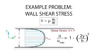
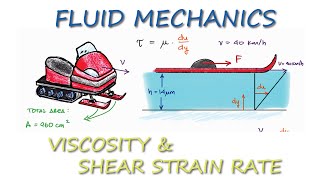
Certainly! The shear stress can be calculated using the formula τ = μ (du/dy).
So what's the summary of what we've discussed?
Wall shear stress arises due to viscous forces against the wall and can be calculated using Navier-Stokes equations.
Velocity Field Calculation
🔒 Unlock Audio Lesson
Sign up and enroll to listen to this audio lesson

Next, let's derive the velocity field using the Navier-Stokes equations. Can anyone recall what assumptions need to be made here?
We need to assume no gravity effect and consider the flow between two fixed parallel plates.
Correct! This leads us to simplify our equations quite a bit. The primary equation we'll use is u = - (dp/dx) * (y^2 / 2μ).
What does each part of that equation mean?
Good question! Here, dp/dx represents the pressure gradient, y is the distance from the centerline, and μ represents dynamic viscosity.
So this equation tells us how velocity varies across the height of the channel?
Absolutely! Now, how can we represent this information visually?
We could draw a graph showing velocity versus the distance from the wall.
Exactly. So what's the key point here?
The velocity field can be calculated using a derived equation from Navier-Stokes under specific conditions.
Vorticity and Velocity Potential Functions
🔒 Unlock Audio Lesson
Sign up and enroll to listen to this audio lesson
Now let's talk about vorticity. Why is it important when calculating wall shear stress?
Vorticity gives us insight into how rotational motion affects the fluid, right?
Yes, and in certain cases, it tells us whether we can find velocity potential functions. Can anyone explain when potential functions can be determined?
Potential functions can be derived when the flow is irrotational.
Exactly! If the vorticity is not zero, we cannot find a velocity potential function. So, why is understanding these relations crucial?
It helps us predict flow behavior under different conditions.
And understanding these concepts applies directly to calculating wall shear stress more effectively!
What’s the take-home message?
Vorticity influences the ability to find potential functions and is essential for understanding wall shear stress in fluid flows.
Average Velocity Calculation
🔒 Unlock Audio Lesson
Sign up and enroll to listen to this audio lesson
Let’s now address the concept of average velocity. How do we compute it in a fluid mechanics context?
We can integrate the velocity field over the flow area and divide by the area?
Exactly! The average velocity (U_avg) can be calculated by integrating u over the area A, which is given by: u_avg = (1/A) * ∫u dA.
What happens to our average velocity if the flow becomes turbulent?
In turbulent flows, the velocity profile is more complex due to fluctuations, so determining an accurate average requires more sophisticated models.
Are there situations where we need to consider dynamic viscosity in these calculations?
Indeed! Viscosity plays a significant role in influencing both the velocity field and the wall shear stress.
So what’s the summary of this discussion?
Average velocity is essential in characterizing fluid flows, calculated by integrating the velocity across an area, considering various scenarios related to flow type and viscosity.
Introduction & Overview
Read summaries of the section's main ideas at different levels of detail.
Quick Overview
Standard
In this section, the wall shear stress calculation is explored through the application of the Navier-Stokes equations, including the derivation of velocity fields, stream functions, and vorticity. Key equations governing these concepts are derived, with particular focus on wall shear stress conditions near fixed boundaries.
Detailed
Wall Shear Stress Calculation
In this section, we delve into the calculation of wall shear stress in fluid dynamics, particularly focusing on flows between two parallel plates where a pressure gradient is present. The foundation involves leveraging the Navier-Stokes equations to derive the velocity field, considering factors like pressure gradient and dynamic viscosity.
Key formulas used include:
1. Velocity Field: The velocity field is first determined under the assumption of a negligible gravitational force and a linear velocity profile between the plates.
The relation is formulated as:
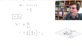
$$ u = - \frac{dp}{dx} \cdot \frac{y^2}{2\mu} + C $$
-
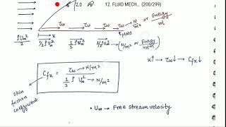
Wall Shear Stress (τ): Wall shear stress is expressed as:
$$ \tau_{xy} = \mu \frac{du}{dy} $$ at the wall (%y = ±h). Deriving this leads to important insights into the distribution of shear stress over the plate's surface. - Stream Functions and Vorticity: The concepts of stream functions and vorticity are also reviewed. The implication of these factors on flow behavior under steady, incompressible conditions is established, with the differentiation highlighting how vorticity affects velocity potential functions.
- Velocity Potential Functions: The prerequisites for obtaining velocity potential functions are stressed, noting their non-existence when flow is rotational.
- Average Velocity: Average velocity across the flow area is computed, taking into account the variables mentioned.
Ultimately, this section offers a comprehensive understanding of wall shear stress calculation through theoretical derivations, practical applications, and assumptions guiding fluid mechanics problems.
Youtube Videos

![[CFD] y+ for Laminar Flow](https://img.youtube.com/vi/yfYr72Gc4S4/mqdefault.jpg)
Audio Book
Dive deep into the subject with an immersive audiobook experience.
Introduction to Wall Shear Stress
Chapter 1 of 6
🔒 Unlock Audio Chapter
Sign up and enroll to access the full audio experience
Chapter Content
This section examines the calculation of wall shear stress and its relation to the velocity field, pressure gradient, and fluid properties.
Detailed Explanation
Wall shear stress is the stress exerted by a fluid on the wall of a channel due to the fluid's viscosity and velocity gradient. In the context of fluid mechanics, it is important to understand how the shear stress is influenced by the velocity field and pressure gradients. The velocity field can be derived using the Navier-Stokes equations, where gravity components may be neglected. The calculation often involves applying Newton's law of viscosity, which relates shear stress to the velocity gradient at the wall.
Examples & Analogies
Think of a river flowing against the bank. The water (fluid) applies force against the bank (wall) due to its movement. The faster the water flows, the more force it exerts on the bank. This is similar to how wall shear stress works.
Calculating Velocity Field
Chapter 2 of 6
🔒 Unlock Audio Chapter
Sign up and enroll to access the full audio experience
Chapter Content
We estimate the velocity field from the Navier-Stokes equations by neglecting gravity, leading to a specific velocity profile dependent on the pressure gradient and viscosity.
Detailed Explanation
The velocity field can be derived from the Navier-Stokes equations by assuming the gravity's effect is negligible. This allows us to simplify the equations to focus on the pressure gradient in the x-direction. The resulting equations give us the velocity profile, where the velocity changes with respect to the vertical coordinate. The differences in flow speeds across the channel contribute to the shear stress experienced at the walls.
Examples & Analogies
Consider a wide flat road where cars are moving at different speeds. The cars on the outer lanes may move faster than those on the inner lanes. Here, the difference in speed creates layers of airflow above the road, similar to how layers of fluid in a channel exhibit different velocities.
Newton's Law of Viscosity Application
Chapter 3 of 6
🔒 Unlock Audio Chapter
Sign up and enroll to access the full audio experience
Chapter Content
To compute wall shear stress, we apply Newton's law of viscosity, which connects shear stress to the velocity gradient at the wall.
Detailed Explanation
Newton’s law of viscosity states that the shear stress between adjacent fluid layers is proportional to the velocity gradient between them. By applying this law at the wall (where one layer is stationary), we can derive expressions for the wall shear stress. In a typical scenario, only the x-component of velocity is relevant at the wall, while the y-component does not contribute since the flow direction is horizontal.
Examples & Analogies
Imagine spreading butter on bread. As you push the knife (representing the fluid) across the surface, the force you apply (shear stress) depends on how quickly you're moving the knife over the butter (the velocity gradient). The faster you move the knife, the more force you need to apply.
Stream Function and Vorticity
Chapter 4 of 6
🔒 Unlock Audio Chapter
Sign up and enroll to access the full audio experience
Chapter Content
In a two-dimensional flow, stream functions can be calculated, which lead us to understand how vorticity interacts in the flow.
Detailed Explanation
The stream function helps visualize two-dimensional, incompressible flows. By defining stream functions, we can derive the flow patterns and study properties like vorticity, which is the measure of the rotation of fluid elements. Vorticity is crucial for understanding how different regions in the flow behave, particularly as flow transitions from laminar to turbulent states.
Examples & Analogies
In a river, water may flow in different patterns where some areas swirl (vorticity) while others flow straight. You can visualize these flows with different streamlines representing paths of water particles.
Average Velocity Calculation
Chapter 5 of 6
🔒 Unlock Audio Chapter
Sign up and enroll to access the full audio experience
Chapter Content
The average velocity is calculated by integrating the velocity field over the cross-sectional area and dividing by that area to yield a mean flow velocity.
Detailed Explanation
The average velocity can be determined by integrating the velocity profile across a specified area and dividing it by that area. This process gives a useful representation of the overall flow behavior despite variations in velocity across different sections of the flow region. Knowing the average velocity is essential for applications in fluid dynamics, ensuring accurate calculations in engineering contexts.
Examples & Analogies
Think about measuring the average speed of cars on a highway. If you observe several cars moving at different speeds and calculate their average, you get a general idea of traffic flow, just like calculating average velocity gives insights into fluid flow dynamics.
Significance of Vorticity and Potential Functions
Chapter 6 of 6
🔒 Unlock Audio Chapter
Sign up and enroll to access the full audio experience
Chapter Content
Vorticity helps understand flow characteristics, especially in irrotational flows where velocity potential functions can be defined.
Detailed Explanation
Vorticity defines regions in the flow where there is rotational motion of fluid particles. In irrotational flows, potential functions arise, which help model velocities without needing to consider rotational effects. When vorticity is present, we can't easily compute potential functions, as their presence violates the assumptions under which potential flows are defined. Understanding these relationships assists in predicting flow behavior and designing systems that effectively manage fluid dynamics.
Examples & Analogies
When a kid spins around very quickly, you can see the whirl of their motion. This is similar to how vorticity works; it illustrates how certain regions of fluid rotate, while in some cases, like water flowing straight down a slide, there is no rotation (no vorticity), illustrating potential flow.
Key Concepts
-
Wall Shear Stress: The shear stress exerted by fluid viscosity at the boundary of flow.
-
Navier-Stokes Equations: Mathematical equations that describe fluid motion and are essential for wall shear stress calculations.
-
Velocity Field: The spatial distribution of fluid velocities, crucial for calculating shear stress.
-
Vorticity: The measure of rotation in fluid flow, influencing velocity potential functions.
-
Average Velocity: A key parameter summarizing flow properties across a defined space.
Examples & Applications
Calculating wall shear stress for fluid flowing between two parallel plates.
Using the Navier-Stokes equations to derive the velocity profile in a channel flow.
Memory Aids
Interactive tools to help you remember key concepts
Rhymes
When fluids flow and near walls cling, wall shear stress is what they'll bring.
Stories
Imagine a river flowing against a cliff; the water struggles to push past, making the cliff feel the force of the flow.
Memory Tools
S.V.A.V: Shear, Viscosity, Average velocity all relate to stress at the wall.
Acronyms
W.S.T = Wall Shear Calculation
What 'S' means Shear
'T' means is the total wall area.
Flash Cards
Glossary
- Wall Shear Stress
The stress induced by the viscous forces in a fluid against the wall of a container or channel.
- NavierStokes Equations
A set of nonlinear partial differential equations that describe the motion of viscous fluid substances.
- Velocity Field
The representation of velocity of fluid at different points in space.
- Vorticity
A measure of the local rotation of the fluid and is a vector field.
- Velocity Potential Function
A scalar function whose gradient gives the velocity field, applicable when the flow is irrotational.
- Dynamic Viscosity
A measure of the fluid's resistance to flow, represented by the symbol μ.
- Average Velocity
The mean velocity of the fluid across a defined area, calculated as the total flow divided by the area.
Reference links
Supplementary resources to enhance your learning experience.