
Velocity Potential Function Discussion
Enroll to start learning
You’ve not yet enrolled in this course. Please enroll for free to listen to audio lessons, classroom podcasts and take practice test.
Interactive Audio Lesson
Listen to a student-teacher conversation explaining the topic in a relatable way.
Understanding Velocity Fields
🔒 Unlock Audio Lesson
Sign up and enroll to listen to this audio lesson

Today, we will be discussing how we derive velocity fields using the Navier-Stokes equations. Can anyone recall what these equations represent in terms of fluid flow?

I think they help describe how fluid velocity changes in different conditions.
Exactly! The Navier-Stokes equations consider the forces acting on the fluid including pressure gradients and viscous forces. When we assume the wall shear stress is zero, we can simplify things significantly. Why do you think that assumption is useful?

It makes the calculations easier since we are ignoring some forces.
Right, simplifying allows us to focus on the primary effects. The simplified equation leads to the expression for the velocity field: u = -dp/dx. Remember, this describes how velocity varies with position along one dimension, enhancing our understanding of the flow. Let's keep this concept in mind.
Wall Shear Stress Relations
🔒 Unlock Audio Lesson
Sign up and enroll to listen to this audio lesson

Now let's discuss wall shear stress. Can anyone tell me how wall shear stress is related to viscosity and velocity gradients?

Isn't it defined using Newton’s law of viscosity, where it relates shear stress to these gradients?
Good catch! The relationship is expressed as τ = μ (du/dy). Here, 'τ' is the shear stress, 'μ' is the dynamic viscosity, and 'du/dy' is the velocity gradient. Hence, as flow near the walls is crucial, the values of 'u' at the walls guide our calculations significantly.

So, if we integrate this across the velocity field, it helps us determine total shear stress?
Exactly! Integrating across the flow field gives us insight into shear stress distributions which are essential for understanding (and predicting!) fluid behavior.
Irrotational Flow and Velocity Potential
🔒 Unlock Audio Lesson
Sign up and enroll to listen to this audio lesson
Next, let's tackle the concept of irrotational flow. What do we mean when we say a flow is irrotational?
It means that the flow doesn't have any vorticity, right?
Exactly! And why is this condition vital for the existence of a velocity potential function?
Because potential functions can only exist when there's no rotation in the flow.
Exactly. If vorticity isn't zero, we can't derive a potential function because it implies that the flow is influenced by rotational forces.
Stream Functions and Averaging Velocities
🔒 Unlock Audio Lesson
Sign up and enroll to listen to this audio lesson
Now, moving on to stream functions, can someone explain how they help in understanding fluid flows?
They allow us to visualize flow patterns, right? It's like mapping out the trajectories of fluid particles.
Spot on! Stream functions are particularly useful in two-dimensional flows as they help to keep track of the flow continuity. To calculate average velocity, we integrate over the area and relate it back to the stream function.
So we get the average velocity by dividing the flow across a defined area?
Correct! And understanding how these concepts interconnect provides a clearer picture of fluid behavior in different scenarios.
Boundary Layers and Their Importance
🔒 Unlock Audio Lesson
Sign up and enroll to listen to this audio lesson
Finally, let’s discuss boundary layers. Why do you think boundary layers are significant in fluid flow?
They can influence drag and lift forces on objects in the flow, like planes and cars!
Exactly! Boundary layers are regions where viscosity controls the flow and are essential for accurate predictions of shear forces acting on surfaces. What happens to flow conditions within these layers?
The velocity gradient is much higher near the wall compared to free stream flow, right?
Exactly! And by understanding boundary layer approximations, we can better solve realistic fluid dynamics problems, leveraging these principles in practical applications.
Introduction & Overview
Read summaries of the section's main ideas at different levels of detail.
Quick Overview
Standard
In this section, we explore the concept of the velocity potential function in the context of fluid mechanics, discussing how it relates to wall shear stress, stream functions, and vorticity in a two-dimensional, incompressible flow scenario. The principles highlighted include the assumptions under the Navier-Stokes equations and the significance of irrotational flow for calculating velocity potential.
Detailed
Detailed Summary
In this section, we dive deep into the velocity potential function, a critical concept in fluid mechanics. The discussion begins by establishing the fundamentals of flow fields, particularly in relation to wall shear stress, stream functions, and vorticity. By negating gravity and applying the Navier-Stokes equations, we derive the velocity fields, particularly focusing on shear stress and the relationship with the pressure gradient.
The concept of shear stress is linked to Newton's laws of viscosity, leading to formulas based on velocity gradients. As the flow is primarily in two dimensions, stream functions can effectively describe the flow. The exploration of vorticity highlights the conditions under which a velocity potential function exists. The necessity of irrotational flow for the potential function is discussed, with clear distinctions made between conditions for its existence and the challenges posed by rotational flow.
Furthermore, average velocity calculations based on area integrations are examined, illustrating the balance of flow across boundaries. The section concludes by emphasizing the challenges presented in fluid flow problems and the crucial role of approximations, particularly in the context of boundary layers created near walls. Overall, it captures the complexity and importance of comprehending velocity potential functions and their mathematical foundations in fluid dynamics.
Youtube Videos

Audio Book
Dive deep into the subject with an immersive audiobook experience.
Understanding Velocity Field and Wall Shear Stress
Chapter 1 of 5
🔒 Unlock Audio Chapter
Sign up and enroll to access the full audio experience
Chapter Content
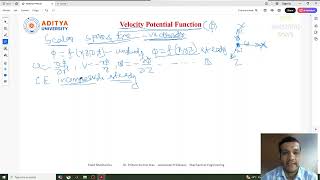
In this discussion, we look at the wall stress, shear stress, stream function, vorticity, velocity potential, and the average velocity, assuming the velocity field is estimated from the Navier-Stokes equations. The velocity field has been calculated neglecting gravity and assuming vw = 0. We derived the u component resulting in a velocity field represented by dp/dx = h²/(2μ)(1 - y²/h²).
Detailed Explanation
This part introduces the relationship between different fluid dynamics properties such as wall shear stress and velocity field calculated using Navier-Stokes equations. Here, 'u' represents the fluid velocity, and the equation describes how this velocity varies based on pressure gradient, dynamic viscosity, and boundary conditions set by wall positions. Essentially, understanding how these factors interplay is vital for analyzing the flow behavior.
Examples & Analogies
Imagine a river flowing smoothly. The speed of water at the center of the river (representing velocity 'u') is faster than that near the riverbank (the wall), due to the friction with the bank that slows it down. Similarly, the derived equation shows how velocity changes within the fluid as it interacts with the boundaries.
Stream Function and Velocity Potential
Chapter 2 of 5
🔒 Unlock Audio Chapter
Sign up and enroll to access the full audio experience
Chapter Content
In this two-dimensional flow, we can calculate stream functions as the flow is steady and incompressible. By integrating the u function, we can find the streamline function considering psi equal to 0 at the centerline. This allows us to estimate the streamline function values at fixed walls, leading to an understanding of stream function relationships.
Detailed Explanation
Stream functions are valuable in fluid mechanics to visualize flow patterns. When dealing with a steady, incompressible flow, you can integrate the velocity function to derive the stream function. By setting conditions like psi = 0 at the centerline, you determine how fluid flows around barriers or surfaces, offering insight into how streamline behavior helps us predict the path of fluid within a given space.
Examples & Analogies
Think of a water slide: as you get closer to the center of the slide, you move faster, which represents the concept of stream functions. Similarly, streamlines help us visualize how water (or another fluid) would behave when flowing around obstacles.
Vorticity and Its Implications
Chapter 3 of 5
🔒 Unlock Audio Chapter
Sign up and enroll to access the full audio experience
Chapter Content
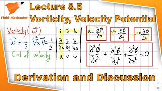
When examining vorticity using curl velocity in the z-direction, we find that for an irrotational flow, vorticity must be zero. Thus, without irrotational flow, calculating velocity potential functions is not feasible, highlighting that potential functions do not exist under certain conditions.
Detailed Explanation
Vorticity measures the local spinning motion of the fluid and plays a critical role in determining flow characteristics. If the flow is irrotational, vorticity equals zero and simplifies the computation of potential functions. However, when fluid experiences rotation or vorticity, these potential functions can't be calculated, illustrating the relationship between rotational dynamics in fluid mechanics.
Examples & Analogies
Imagine a spinning top; its vorticity (the spinning motion) means you can’t predict where it will fall (the velocity potential). Conversely, a still object like a ball resting on the ground doesn’t have such unpredictable motion, making its potential energies computable.
Average Velocity Calculation
Chapter 4 of 5
🔒 Unlock Audio Chapter
Sign up and enroll to access the full audio experience
Chapter Content
We can compute average velocity by calculating the discharge related to the velocity field from minus h to plus h over the area. This involves integrating the velocity field from placed boundaries, leading to the average velocity in fluid flow scenarios.
Detailed Explanation
Calculating average velocity involves integrating the velocity distribution over a specified cross-sectional area. When evaluating the velocity fields, taking into account the changes from the lowest to the highest flow (minus h to plus h) allows for understanding how fluid behaves as a whole rather than at isolated points.
Examples & Analogies
Think about measuring the flow rate of water in a garden hose. By observing how much water flows out over a period—across the entire diameter of the hose—you calculate the average speed of water rather than focusing on the flow at just a single point.
Importance of Navigation Using Navier-Stokes Equations
Chapter 5 of 5
🔒 Unlock Audio Chapter
Sign up and enroll to access the full audio experience
Chapter Content
Utilizing the Navier-Stokes equations helps us estimate various flow criteria, including wall shear stress, stream functions, and more. The comparison to integral approaches is drawn, emphasizing the complexity involved in differential methods, where a series of approximations are essential.
Detailed Explanation
The Navier-Stokes equations encapsulate the principles of fluid motion, imparting critical insights into various flow fields. By applying these equations, engineers and scientists can forecast how different forces and constraints affect fluid behavior, although deriving solutions can be complex compared to simpler integral methods.
Examples & Analogies
Imagine navigating through a busy city with a map (the Navier-Stokes equations). Understanding each road's twists and turns makes it complex, just like calculating fluid dynamics; however, knowing shortcuts can simplify the journey, similar to the easier approaches in integral methods.
Key Concepts
-
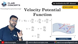
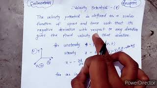
Velocity Potential Function: A function that defines the velocity field in an irrotational flow.
-
Wall Shear Stress: Shear stress at the boundaries of turbulent flows, calculated using viscosity laws.
-
Vorticity: The rotational component of the velocity field, crucial for defining flow behavior.
-
Stream Functions: Functions that represent flow patterns in incompressible two-dimensional flow.
-
Boundary Layers: Regions in fluid flow near surfaces where viscosity dominates, affecting shear and flow characteristics.
Examples & Applications
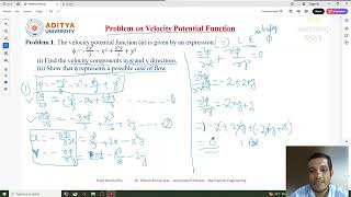
When calculating wall shear stress using the Navier-Stokes equations, integrating velocity gradients can show strong reliance on viscosity.
In two-dimensional flow scenarios, analyzing stream functions can reveal how velocity changes across the flow field.
Memory Aids
Interactive tools to help you remember key concepts
Rhymes
Shear stress at the wall, viscosity is the call. In fluid flow, both rise and fall.
Stories
Imagine a water slide where the water moves quickly at the top but slows down at the bottom due to friction against the slide. This friction is like wall shear stress acting due to viscosity.
Memory Tools
To remember the conditions for velocity potential: IRR (Irrotational, Simple, Reflective).
Acronyms
VWS (Velocity, Wall shear stress) helps remember the relationship between velocity fields and wall shear calculations.
Flash Cards
Glossary
- Velocity Potential Function
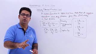
A scalar function whose gradient gives the velocity field of an incompressible and irrotational flow.
- Wall Shear Stress
The stress exerted by a fluid on the boundary wall of its flow due to viscosity.
- Vorticity
A measure of the rotation of fluid elements in a flow field, representing the local spinning motion.
- Stream Function
A mathematical tool used to visualize flow patterns, especially in two-dimensional incompressible flows.
- Average Velocity
The mean flow velocity over a defined area, usually calculated through integration across the flow domain.
Reference links
Supplementary resources to enhance your learning experience.