
Approximate solutions using CFD
Enroll to start learning
You’ve not yet enrolled in this course. Please enroll for free to listen to audio lessons, classroom podcasts and take practice test.
Interactive Audio Lesson
Listen to a student-teacher conversation explaining the topic in a relatable way.
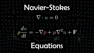
Introduction to Navier-Stokes Equations
🔒 Unlock Audio Lesson
Sign up and enroll to listen to this audio lesson

Good morning everyone! Today, we're going to delve deeper into the Navier-Stokes equations. Can anyone remind me why these equations are crucial in fluid dynamics?

They describe how fluids move and interact, right?
Exactly! They encompass mass conservation and momentum equations. How do we approach solving them, particularly for simplified cases?

We can apply some assumptions and approximations, like assuming constant viscosity?
Yes! By assuming constant viscosity and incompressibility, we can simplify the equations significantly. Remember the acronym 'IC' for Incompressible, and 'C' for Constant viscosity!

Does that mean we can find approximate solutions even when the flow is turbulent?
Great question! While turbulent flows are complex, modern methods like Computational Fluid Dynamics (CFD) allow us to simulate these flows. Who can remind us of the main components involved in these equations?

Local acceleration, convective acceleration, pressure gradients, and viscosity!
Right again! Understanding these terms will help us navigate through the calculations involved. Let's reconvene this later.
Simplifying Complex Equations
🔒 Unlock Audio Lesson
Sign up and enroll to listen to this audio lesson

Now, let's focus on how we can simplify Navier-Stokes equations for specific cases. What happens when we assume that the viscosity is almost zero?
We can derive Euler's equations, right?
Correct! Euler's equations are simpler and applicable when viscous effects are negligible. Can anyone list the assumptions we use in deriving Euler's equations?
Incompressibility, no viscosity, and steady flow conditions?
Nailed it! And under what conditions do we often apply Bernoulli's equation?
When flow is along streamlines and under steady, frictionless conditions.
Exactly! Just remember the 'S' in Bernoulli's for 'Streamlines.' This leads us to the derivations we explore next. Let's take a look at some examples.
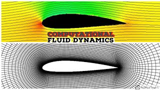
Computational Fluid Dynamics (CFD)
🔒 Unlock Audio Lesson
Sign up and enroll to listen to this audio lesson
Now, who here is familiar with Computational Fluid Dynamics, or CFD?
I've heard of it. It’s a method to simulate fluid flows and solve the equations numerically, right?
Yes! CFD represents how we can tackle complex flows that defy simple analytical solutions. Now, why do we rely on approximations in CFD?
Because real-world flows can be incredibly complex, like turbulence and varying temperatures.
Precisely! The more complex the flow, the greater the need for approximations through CFD. How do we represent these approximations?
By using numerical methods and setting appropriate boundary conditions!
Exactly! Using techniques like discretization, we can make fluid problems solvable. Let’s consider a practical example to reinforce this.
Practical Applications of CFD
🔒 Unlock Audio Lesson
Sign up and enroll to listen to this audio lesson
Our next topic involves practical applications: Can anyone think of industries where fluid dynamics—particularly CFD—is applied?
Everywhere in civil engineering, especially in designing hydraulic systems!
Also in aerospace for analyzing airflow over wings!
Absolutely! CFD has significant implications. It's not just theoretical; applications range from biomedical to environmental engineering. Can anyone think of an example where approximations in fluid dynamics are crucial?
Like in analyzing blood flow in arteries! Accurate simulations can help in medical diagnostics.
Wonderful connection! Understanding these simulations enhances our comprehension of fluid flows and their controlling factors. Let's summarize our insights from today.
Introduction & Overview
Read summaries of the section's main ideas at different levels of detail.
Quick Overview
Standard
In this section, the importance of approximations in the Navier-Stokes equations is explored, particularly through the lens of incompressible flow conditions. The discussion highlights methodologies such as assuming constant viscosity and simplifying terms to enable analytical solutions or computational fluid dynamics approaches, especially when dealing with complex flow scenarios like turbulence.
Detailed
Detailed Summary
In this section, the fundamental principles of approximate solutions to the Navier-Stokes equations are examined, particularly within the realm of Computational Fluid Dynamics (CFD). The Navier-Stokes equations describe the motion of fluid substances, relying on core assumptions like incompressibility, constant density, and constant viscosity to simplify the equations into a more manageable form. Through discussions of local and convective acceleration, pressure gradients, and various fluid flow conditions, the complexity of turbulence and energy conservation is acknowledged.
The section also emphasizes how CFD has transformed fluid mechanics by allowing for the numerical solution of these equations under various initial and boundary conditions. It is noted that simplifications are critical in deriving analytical solutions such as Bernoulli's equation from Euler equations, and numerous real-world examples are provided to illustrate how these principles are applied across different fields including civil engineering and biomechanics. The importance of recognizing the conditions under which viscosity and flow characteristics change is highlighted, paving the way for further exploration of the Navier-Stokes framework in more advanced studies.
Youtube Videos
![[CFD] Inflation Layers / Prism Layers in CFD](https://img.youtube.com/vi/1gSHN99I7L4/mqdefault.jpg)

![[CFD] The Finite Volume Method in CFD](https://img.youtube.com/vi/E9_kyXjtRHc/mqdefault.jpg)
![[CFD] Pseudo Transients for Steady-State CFD (Part 1) - Pseudo vs True Transients](https://img.youtube.com/vi/rF2t0-JmQZg/mqdefault.jpg)


![[CFD] Residuals in CFD (Part 1) - Understanding Residuals](https://img.youtube.com/vi/v9OnNeYH4Ok/mqdefault.jpg)
Audio Book
Dive deep into the subject with an immersive audiobook experience.
Introduction to Approximate Solutions
Chapter 1 of 5
🔒 Unlock Audio Chapter
Sign up and enroll to access the full audio experience
Chapter Content
Now, if you will go for the next part which is the boundary conditions which I just introduced to you that first conditions is no slip boundary condition.
Detailed Explanation
This chunk introduces the concept of approximate solutions in the context of Computational Fluid Dynamics (CFD). Approximations are necessary because solving the Navier-Stokes equations directly can be quite complex, especially for turbulent flows. The text mentions that while CFD can provide approximate results, it is essential to apply appropriate assumptions and boundary conditions to simplify these equations and derive useful solutions.
Examples & Analogies
Think of it like using a GPS to chart a course. The GPS simplifies the routes you can take by considering traffic assumptions and road conditions, which is much like how CFD simplifies fluid dynamics problems to find approximate solutions based on set conditions.
Conditions for Approximate Solutions
Chapter 2 of 5
🔒 Unlock Audio Chapter
Sign up and enroll to access the full audio experience
Chapter Content
So if I just want to draw the streamline of these flow patterns, even if I do not solve it, if I just used a streamline, so I can draw a streamlines.
Detailed Explanation
This chunk emphasizes using streamlines to visualize flow patterns without necessarily solving complex equations. Streamlines represent the paths followed by particles in the fluid flow, and can help predict velocity distributions and behaviors in various fluid scenarios. This visualization can often lead to understanding and simplifying the problem at hand.
Examples & Analogies
Imagine observing a river: you can see how the water flows around obstacles like rocks by looking at the surface at any moment. This observation gives you an understanding of the current without needing to dredge up all the physics behind the flow.
Role of Boundary Conditions
Chapter 3 of 5
🔒 Unlock Audio Chapter
Sign up and enroll to access the full audio experience
Chapter Content
As I discuss it that We will not look it to solve this Navier-Stokes equations as it because it is a non-linear two-dimensional equations.
Detailed Explanation
Boundary conditions are crucial for solving fluid dynamics problems because they define how the fluid behaves at the limits of the flow domain. The text introduces the notion of no-slip boundary conditions, which are standard in fluid mechanics, especially when dealing with viscous flows. These conditions state that the velocity of the fluid at the boundary is equal to the velocity of the boundary itself, usually set to zero for stationary walls.
Examples & Analogies
Consider a car moving through a tunnel. The air right next to the tunnel walls doesn't move; it stays stagnant while the car (the boundary) moves through it. This is akin to the no-slip condition, where the fluid at the boundary remains fixed, mirroring the condition at the walls of a pipe or channel.
Transitioning to Simplified Equations
Chapter 4 of 5
🔒 Unlock Audio Chapter
Sign up and enroll to access the full audio experience
Chapter Content
We try to simplify these equations.
Detailed Explanation
This chunk highlights the transition from more complex equations (like the Navier-Stokes) to simpler forms (like the Euler equations). The goal is to achieve a set of relationships that can be solved more easily or approximated effectively. This approach enables engineers to predict fluid behavior without getting bogged down by overly detailed calculations that are often impractical.
Examples & Analogies
Think about a teacher trying to explain a complex math problem to students. Instead of delving into every single detail (which might confuse students), the teacher simplifies the problem to the core concepts, allowing students to grasp essential techniques before tackling the more complex aspects.
Application of Computational Fluid Dynamics
Chapter 5 of 5
🔒 Unlock Audio Chapter
Sign up and enroll to access the full audio experience
Chapter Content
But if you look at these terms, if I look at this d v by d t, if I just expand it I will have a in vector forms.
Detailed Explanation
This part discusses how when expanding these equations in vector forms, CFD can be leveraged to approximate the solutions of velocity, pressure, and other key parameters in fluid systems. It underscores that instruments such as computational simulations help visualize complex fluid behaviors that would otherwise require significant mathematical manipulation.
Examples & Analogies
Imagine using weather simulation software that predicts weather patterns based on numerous variables. It simplifies and models these real-world conditions, much like CFD simplifies fluid dynamics problems, allowing scientists to visualize and predict fluid flows efficiently.
Key Concepts
-
Navier-Stokes Equations: Fundamental equations describing fluid motion based on conservation laws.
-
Computational Fluid Dynamics (CFD): Numerical analysis of fluid flows utilizing algorithms and computational power.
-
Incompressibility: Key assumption simplifying fluid dynamics, particularly in water flows.
-
Local vs. Convective Acceleration: Two types of acceleration affecting fluid particle movement.
-
Turbulent Flow: More complex flow regimes characterized by chaotic changes in pressure and velocity.
Examples & Applications
Blood flow analysis in arteries using CFD to understand blockage effects.
Simulating airflow over aircraft wings to enhance aerodynamic performance.
Analysis of river flows around structures like bridges to reduce erosion risks.
Memory Aids
Interactive tools to help you remember key concepts
Rhymes
To flow it right, keep velocity in sight, Navier-Stokes will guide through fluid’s flight.
Stories
Imagine a fluid flowing smoothly, dancing in a river. Each data point represents a speed, helping engineers design bridges. Remember flow continuity for smooth sailing.
Memory Tools
IC stands for Incompressibility and Constant viscosity, essential for simplifying Navier-Stokes.
Acronyms
B.E.S.T. - Bernoulli’s Equations under Steady flow and Turbulence are key assumptions.
Flash Cards
Glossary
- NavierStokes Equations
Equations that describe the motion of fluid substances using principles of motion and conservation of mass.
- Computational Fluid Dynamics (CFD)
A numerical method used to analyze fluid flows and solve the Navier-Stokes equations using computers.
- Incompressibility
Assumption that density remains constant in fluid flow scenarios, simplifying the Navier-Stokes equations.
- Local Acceleration
Rate of change of velocity of a fluid particle with respect to time at a fixed point.
- Convective Acceleration
Rate of change of velocity of a fluid particle due to the movement of the fluid itself.
Reference links
Supplementary resources to enhance your learning experience.