
Assumptions in fluid equations
Enroll to start learning
You’ve not yet enrolled in this course. Please enroll for free to listen to audio lessons, classroom podcasts and take practice test.
Interactive Audio Lesson
Listen to a student-teacher conversation explaining the topic in a relatable way.
Introduction to Fluid Equations
🔒 Unlock Audio Lesson
Sign up and enroll to listen to this audio lesson

Good morning, class! Today we are discussing the fundamental assumptions involved in fluid equations, specifically the Navier-Stokes equations. Can anyone tell me why we need assumptions in these equations?

To simplify the equations and make them easier to solve?
Exactly! Assumptions allow us to reduce complexity. For example, one key assumption is incompressibility. Who can explain what that means?

It means the density of the fluid remains constant during flow.
Correct! This assumption is crucial for simplifying mass conservation equations. Remember, we use the acronym 'IC' for Incompressible Constant!
Newtonian Fluids
🔒 Unlock Audio Lesson
Sign up and enroll to listen to this audio lesson

Now, let's dive into the second assumption: the fluid must behave like a Newtonian fluid. What does that entail?

It means there's a linear relationship between shear stress and the velocity gradient?
Spot on! This means that the viscosity remains constant under the conditions we consider. What might happen if the fluid were non-Newtonian?

Then the equations would get much more complex, right? Viscosity could change with different flow conditions.
Exactly! And for clarity, let's use the mnemonic 'VIC' for Viscosity In Control. Good job!
Significance of Isothermal Conditions
🔒 Unlock Audio Lesson
Sign up and enroll to listen to this audio lesson
Finally, we address the assumption of isothermal conditions. Why is this important in fluid dynamics?
"Because it keeps the viscosity constant?
Numerical Methods vs Analytical Solutions
🔒 Unlock Audio Lesson
Sign up and enroll to listen to this audio lesson
As we apply these assumptions, we often find ourselves choosing between analytical solutions and numerical methods. What would be the advantage of focusing on analytical solutions?
They can provide exact solutions for specific conditions and show how flow variables relate!
Exactly! Analytical solutions are crucial for understanding system behavior. However, when dealing with complex scenarios, what are our options?
We could use computational fluid dynamics, right? It handles complex geometries and non-linear behaviors.
Very good! Computational fluid dynamics helps when analytical methods fall short. Always remember: 'Simplicity Over Complexity' when studying fluid mechanics.
Review of Assumptions
🔒 Unlock Audio Lesson
Sign up and enroll to listen to this audio lesson
To wrap up, let's summarize what we've learned about the assumptions in fluid equations. Starting with incompressibility, can someone explain it once more?
Incompressibility means fluid density is constant, which simplifies mass conservation.
Correct! Next, how about the Newtonian fluid assumption?
It states there's a constant relationship between shear stress and velocity gradient.
Exactly! And finally, why do we need isothermal conditions?
To keep viscosity constant, ensuring simplified solutions can be derived.
Well done, everyone! Always focus on these key assumptions as the foundation for understanding fluid dynamics.
Introduction & Overview
Read summaries of the section's main ideas at different levels of detail.
Quick Overview
Standard
In this section, we explore the key assumptions underlying the Navier-Stokes equations, including the incompressibility, Newtonian fluid behavior, and isothermal conditions. These assumptions simplify the equations and facilitate analytical solutions for fluid flows, highlighting how neglecting certain terms influences outcomes in fluid mechanics.
Detailed
Assumptions in Fluid Equations
There are several critical assumptions when deriving fluid equations, particularly the Navier-Stokes equations, which are pivotal in fluid mechanics. In this section, we focus on three main assumptions:
- Incompressibility: The fluid density is approximately constant, which simplifies the equations used to describe mass conservation.
- Newtonian Fluid: The relationship between shear stress and velocity gradient is linear; that is, the viscosity remains constant under a range of conditions (specifically, isothermal conditions).
- Isothermal Conditions: The temperature of the fluid does not change significantly during flow, maintaining constant viscosity.
The implications of these assumptions are profound; they allow the Navier-Stokes equations to be simplified and manipulated into forms that can yield analytical solutions for various fluid dynamics scenarios. For instance, under conditions where viscosity is negligible, the equations can reduce to the Euler equations.
Additionally, the section emphasizes how understanding these assumptions not only helps in deriving fundamental equations like the Bernoulli equations but also aids in recognizing the limitations of these models in real-world applications.
Youtube Videos
![Common assumptions in fluid mechanics [Fluid Mechanics #3b]](https://img.youtube.com/vi/kimMbNP9DrY/mqdefault.jpg)


Audio Book
Dive deep into the subject with an immersive audiobook experience.
Basic Assumptions in Fluid Mechanics
Chapter 1 of 7
🔒 Unlock Audio Chapter
Sign up and enroll to access the full audio experience
Chapter Content
Please always have a remember what are the assumptions we have when you are deriving basic fluid equations today as we are discussing about Navier-Stokes equations.
Detailed Explanation
Fluid mechanics relies on certain foundational assumptions when working with fluid equations, particularly the Navier-Stokes equations. These assumptions shape how we interpret fluid behavior and simplify complex phenomena into manageable equations. Understanding these assumptions is crucial for applying fluid mechanics effectively.
Examples & Analogies
Think of it like baking a cake. When a baker assumes certain things—like the ideal temperature of the oven and the freshness of the ingredients—they can create a delicious cake. Similarly, in fluid mechanics, these assumptions help 'bake' simpler equations from complex realities.
Characteristics of Newtonian Fluids
Chapter 2 of 7
🔒 Unlock Audio Chapter
Sign up and enroll to access the full audio experience
Chapter Content
So, we have considered the isothermal case where the viscosity (mu) is a constant. We have considered incompressible flow where the density (rho) is a constant.
Detailed Explanation
When working with the Navier-Stokes equations, ideal fluids are often categorized as Newtonian fluids. These fluids exhibit a constant viscosity (mu), regardless of the flow conditions. Additionally, incompressible flow assumes that the density (rho) of the fluid remains constant. These characteristics simplify the equations significantly.
Examples & Analogies
Imagine honey flowing smoothly in a jar—its viscosity stays the same regardless of how fast you pour it. This behavior is similar to that of a Newtonian fluid. In contrast, think of a scenario where you quickly shake a can of soda; the carbon dioxide bubbles change the fluid's compressibility, which complicates the situation!
Local and Convective Accelerations
Chapter 3 of 7
🔒 Unlock Audio Chapter
Sign up and enroll to access the full audio experience
Chapter Content
So, this is the local acceleration, this is the convective acceleration.
Detailed Explanation
In fluid dynamics, acceleration can be classified as local or convective. Local acceleration refers to changes in velocity at a specific point in space over time, while convective acceleration involves changes in velocity due to the motion of the fluid itself. Understanding these types of acceleration is essential for analyzing how fluids move and interact within a given system.
Examples & Analogies
Consider a subway train: local acceleration is like the moment when the train speeds up just as you are getting on, while convective acceleration is akin to the overall speed changes as the train moves through the city. Both contribute to your experience, just as local and convective acceleration do in fluid flow!
Pressure Gradients and Forces
Chapter 4 of 7
🔒 Unlock Audio Chapter
Sign up and enroll to access the full audio experience
Chapter Content
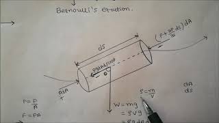
We have a pressure gradient part, we have a gravity force and we have the Laplacian operator of the velocity in the u directions.
Detailed Explanation
The Navier-Stokes equations account for various forces acting on a fluid element, including pressure gradients and gravity. The pressure gradient drives fluid flow, while gravitational force influences the direction and acceleration of the fluid. The Laplacian operator essentially describes how the velocity field varies across space, further complicating the fluid's behavior.
Examples & Analogies
Think of a water slide: the pressure at the top pushes you down the slide (pressure gradient), gravity pulls you downward, enhancing your speed, and the curve of the slide represents how the speed changes due to varying angles (Laplacian operator). These forces together create a thrilling ride!
Simplifying the Navier-Stokes Equations
Chapter 5 of 7
🔒 Unlock Audio Chapter
Sign up and enroll to access the full audio experience
Chapter Content
How I can simplify these equations for examples if I consider the mu is very very close to 0.
Detailed Explanation
In fluid mechanics, simplifying the Navier-Stokes equations is crucial for obtaining practical solutions. By scrutinizing and adjusting various parameters—like setting viscosity (mu) to near zero—physicists can derive more manageable forms of these equations under specific conditions, leading to simplified models like the Euler equations.
Examples & Analogies
Imagine trying to play a video game while it’s running too slowly; simplifying your settings may allow for a smoother experience without losing the fun of the game. Similarly, fluid mechanics 'simplifies' complex equations to play the dynamics of fluids more effectively!
Euler Equations and Their Applications
Chapter 6 of 7
🔒 Unlock Audio Chapter
Sign up and enroll to access the full audio experience
Chapter Content
If these terms are 0 in a particular fluid flow, then these equations become a very linear form of very simplified equations that is what we called the Euler equations.
Detailed Explanation
Euler equations emerge from the simplification of Navier-Stokes equations where viscous forces become negligible. These equations describe the motion of an inviscid (non-viscous) fluid, allowing for a linear, more manageable form. Understanding where and how to apply Euler equations is vital for engineers and scientists working with fluids.
Examples & Analogies
Think of a perfectly smooth ski slope where friction is minimal—the skier glides along easily, similar to how the Euler equations describe an ideal fluid. In real world scenarios, however, most slopes (or fluids) will experience some friction or resistance!
Complex Cases and Computational Fluid Dynamics
Chapter 7 of 7
🔒 Unlock Audio Chapter
Sign up and enroll to access the full audio experience
Chapter Content
No doubt, today we have computational fluid dynamics with us. We can solve this equation.
Detailed Explanation
Today, complex fluid flow problems are often tackled using computational fluid dynamics (CFD), where powerful computers simulate fluid behavior under a variety of conditions. CFD takes into account all factors, such as viscosity and turbulence, which were previously too complex to analyze using traditional analytical methods.
Examples & Analogies
Consider a filmmaker creating a movie with special effects—the realism of flying dragons or underwater scenarios requires advanced software to simulate these effects accurately. Similarly, CFD allows scientists to visualize and understand fluid dynamics in all their complex glory.
Key Concepts
-
Incompressibility: Fluid density is constant.
-
Newtonian Fluid: Shear stress vs. velocity gradient.
-
Isothermal Conditions: Temperature does not significantly vary.
-
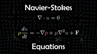
Navier-Stokes Equations: Describe fluid motion.
-
Simplifications: Leading to analytical and numerical solutions.
Examples & Applications
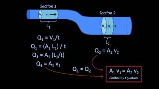
An incompressible flow of water in a pipe where the density remains constant.
A scenario where temperature changes lead to variable viscosity in a non-Newtonian fluid.
Memory Aids
Interactive tools to help you remember key concepts
Rhymes
If density flows in a constant space, that makes incompressibility a valid case.
Stories
Imagine riding a bicycle in a straight line (the flow) on a flat road (the incompressible assumption) - moving at a constant speed, so your ride is easy without bumps (constant density).
Memory Tools
ICN for Incompressibility, Constant Viscosity, Newtonian Fluid.
Acronyms
IVI for Isothermal Viscosity Is constant.
Flash Cards
Glossary
- Incompressibility
Assumption that the fluid density remains constant during flow.
- Newtonian Fluid
A fluid in which the relationship between shear stress and the velocity gradient is linear.
- Isothermal Conditions
Assumption that there are no significant temperature variations affecting fluid behavior.
- NavierStokes Equations
Equations that describe the motion of viscous fluid substances.
- Euler Equations
Simplified equations derived from the Navier-Stokes equations under certain assumptions, ignoring viscosity.
- Bernoulli's Equation
A principle that describes the conservation of energy in fluid flow under specific conditions.
Reference links
Supplementary resources to enhance your learning experience.