
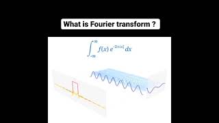
Solving Differential Equations Using Fourier Transform
Enroll to start learning
You’ve not yet enrolled in this course. Please enroll for free to listen to audio lessons, classroom podcasts and take practice test.
Interactive Audio Lesson
Listen to a student-teacher conversation explaining the topic in a relatable way.
Understanding the Differential Equation
🔒 Unlock Audio Lesson
Sign up and enroll to listen to this audio lesson

Today we'll discuss a second-order linear ordinary differential equation. It usually takes the form 'd²y/dt² - 3dy/dt + 2y = f(t)'. Can anyone tell me the components of this equation?

The components are the second and first derivatives of y, as well as the function f(t) on the right side.
That's correct! The left side represents the behavior of the system, while f(t) is the external force acting upon it. What might be the challenge in solving this directly?

It seems complex; we need to find y for every t.
Exactly! That's where the Fourier Transform comes in handy. It helps convert our equation into a more manageable form in the frequency domain.
Fourier Transform Application
🔒 Unlock Audio Lesson
Sign up and enroll to listen to this audio lesson

Now, let's apply the Fourier Transform to both sides of our ODE. We have 'F{d²y/dt²} - 3F{dy/dt} + 2F{y} = F{f(t)}'. Does anyone remember how to transform derivatives using Fourier?

Yes! The Fourier Transform of a derivative brings in factors of iω.
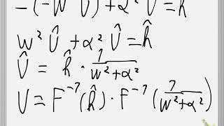
Right on! That means we rewrite the equation as '(-ω²Y(ω)) - 3(iωY(ω)) + 2Y(ω) = F(ω)'. What does this form allow us to do?

It lets us solve for Y(ω) conveniently!
Exactly! Next, we'll manipulate that equation to express Y(ω) in terms of F(ω).
Solving for Y(ω)
🔒 Unlock Audio Lesson
Sign up and enroll to listen to this audio lesson
Let's rearrange our equation: 'Y(ω) = F(ω)/(-ω² - 3iω + 2)'. What insight does this give us?
It shows how the frequency response of our input f(t) determines the output Y(ω).
That's correct! The behavior of y is entirely defined in terms of the function F(ω), which represents our initial disturbance. Finally, what do we do to find y(t)?
We take the inverse Fourier Transform.
Precisely! This completes our solution process for the differential equation using the Fourier Transform.
Applications in Engineering
🔒 Unlock Audio Lesson
Sign up and enroll to listen to this audio lesson
We have now learned how to solve a differential equation using Fourier Transform. Why is this important for engineering applications?
It simplifies the analysis of dynamic systems, like vibrations and heat conduction.
Absolutely! Many engineering problems can be complex in the time domain but become more manageable when analyzed in the frequency domain. Let's think about how we might apply this knowledge practically.
For example, when designing structures, we need to understand how they respond to dynamic loads.
Exactly! This knowledge equips engineers to create safer and more efficient systems.
Introduction & Overview
Read summaries of the section's main ideas at different levels of detail.
Quick Overview
Standard
In this section, we learn how the Fourier Transform can be applied to solve second-order linear ordinary differential equations (ODEs). By transforming the ODEs into the frequency domain, we simplify the process of finding solutions, especially in engineering fields. The methodology involves taking the Fourier Transform of both sides of the equation, allowing us to express the solution in terms of its Fourier Transform.
Detailed
Detailed Summary
In this section, we explore the application of the Fourier Transform to solve second-order linear ordinary differential equations (ODEs). These equations often appear in engineering problems related to vibrations, heat transfer, and signal processing.
Key Steps in Solving a Differential Equation with Fourier Transform:
- Start with the Second-Order Linear ODE
- We consider an equation of the form: $$\frac{d^2y}{dt^2} - 3\frac{dy}{dt} + 2y = f(t)$$
- Take the Fourier Transform of Both Sides
- Applying the Fourier Transform allows us to switch from the time domain to the frequency domain: $$F\left\{\frac{d^2y}{dt^2} \right\} - 3F\left\{\frac{dy}{dt} \right\} + 2F\{y\} = F\{f(t)\}$$
- Utilize Differentiation Properties of the Fourier Transform
- Using the property that relates differentiation in the time domain to multiplication by $i\omega$ in the frequency domain, we rewrite the equation as: $$(-\omega^2Y(\omega)) - 3(i\omega Y(\omega)) + 2Y(\omega) = F(\omega)$$
- Solve for $Y(\omega)$
- Rearranging gives: $$Y(\omega) = \frac{F(\omega)}{-\omega^2 - 3i\omega + 2}$$
- Inverse Transform
- Finally, we take the inverse Fourier Transform to find $y(t)$, completing the solution process.
This method is particularly useful in boundary value problems where finding Green’s functions can be complicated.
Youtube Videos
Audio Book
Dive deep into the subject with an immersive audiobook experience.
Introduction to the Differential Equation
Chapter 1 of 4
🔒 Unlock Audio Chapter
Sign up and enroll to access the full audio experience
Chapter Content
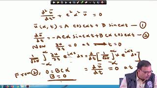
Let us consider a second-order linear ODE:
d²y
dy
−3 +2y =f(t)
dt²
dt
Detailed Explanation
This chunk introduces a second-order linear ordinary differential equation (ODE) that we will solve using Fourier transforms. The equation involves second derivatives (d²y/dt²) and first derivatives (dy/dt) of the function y, with an arbitrary function f(t) acting as the input or forcing function to the system. The ODE represents a common form encountered in various applications, including physics and engineering.
Examples & Analogies
Think of this equation as describing the motion of a spring-mass system where the spring experiences an external force f(t). The terms involving derivatives represent how the system's position changes over time, akin to a car's acceleration and velocity changes when it brakes.
Applying Fourier Transform
Chapter 2 of 4
🔒 Unlock Audio Chapter
Sign up and enroll to access the full audio experience
Chapter Content
Taking the Fourier Transform of both sides:
(cid:26) d²y(cid:27) (cid:26) dy(cid:27)
F −3F +2F{y}=F{f(t)}
dt²
dt
Detailed Explanation
This step applies the Fourier Transform to the entire differential equation. The Fourier Transform converts the time domain expressions (the derivatives with respect to time) into frequency domain representations by replacing derivatives with algebraic terms. The left side of the equation now features transformed variables (like F{y} for y) with derivatives represented in terms of frequency ω. This manipulation simplifies the equation into an algebraic form, making it easier to solve.
Examples & Analogies
Imagine transforming your favorite recipe from a long, detailed set of instructions (time domain) into a concise list of ingredients and steps (frequency domain). Just as it's easier to manipulate a shopping list than a full cooking guide, it becomes simpler to solve mathematical problems in this new form.
Rearranging Terms
Chapter 3 of 4
🔒 Unlock Audio Chapter
Sign up and enroll to access the full audio experience
Chapter Content
⇒(−ω²Y(ω))−3(iωY(ω))+2Y(ω)=F(ω)
Y(ω)(−ω²−3iω+2)=F(ω)⇒Y(ω)=
F(ω)
−ω²−3iω+2
Detailed Explanation
After applying the Fourier Transform, we rearrange the terms to isolate Y(ω), which represents the Fourier transform of the function y(t). The equation reveals how Y(ω) is expressed in relation to F(ω), the Fourier Transform of the input function. This enables us to express the solution to the differential equation in the frequency domain, simplifying analysis of its behavior.
Examples & Analogies
Consider a puzzle that needs rearranging. Just like you would group pieces by color or edge shape to solve it more easily, rearranging the equation facilitates isolating the solution variables, making it easier to work towards finding the final solution.
Inverse Transform for Solution
Chapter 4 of 4
🔒 Unlock Audio Chapter
Sign up and enroll to access the full audio experience
Chapter Content
Take the inverse transform of Y(ω) to get y(t).
This approach is crucial for solving boundary value problems, especially where Green’s functions are hard to construct.
Detailed Explanation
The final step involves taking the inverse Fourier Transform of Y(ω) to revert from the frequency domain back to the time domain, providing the solution for y(t). This capability to convert between domains is essential in solving boundary value problems and is particularly valuable in engineering fields where traditional methods may be complex or unwieldy.
Examples & Analogies
Imagine receiving a package containing a complex structure in pieces; using the transform is like having assembly instructions that allow you to understand how to put it all together. The inverse transform provides you with clear directions to reconstruct your original output, just as following instructions helps you build the intended model from scattered parts.
Key Concepts
-
Fourier Transform: A technique used to convert a function of time into a function of frequency.
-
Linear ODE: An ordinary differential equation in which the unknown function and its derivatives appear linearly.
-
Frequency Domain: A perspective for analyzing functions using frequency instead of time.
-
Inverse Transform: The operation that converts transformed data back to its original form.
Examples & Applications
Solving the differential equation d²y/dt² - 3dy/dt + 2y = f(t) using Fourier Transform.
The application of Fourier analysis in designing control systems.
Using the Fourier Transform to analyze mechanical vibrations in engineering.
Memory Aids
Interactive tools to help you remember key concepts
Rhymes
In transforms where functions play, derivatives will fade away.
Stories
Imagine a busy city where cars (representing functions) change their paths when entering a tunnel (the Fourier Transform) that leads them into a serene park (the frequency domain). Inside the park, it's easier to manage traffic (solving the equation).
Memory Tools
TSY - Transform, Solve, Yield. Remember these steps to find Y(ω)!
Acronyms
ODE - Ordinary Differential Equations
their analysis can lead to Direct answers in the frequency domain.
Flash Cards
Glossary
- Ordinary Differential Equation (ODE)
A differential equation containing one or more functions of one independent variable and its derivatives.
- Fourier Transform
A mathematical transform that expresses a function in terms of its frequency components.
- Frequency Domain
A representation of a signal or function in terms of frequency, rather than time.
- Inverse Fourier Transform
A process that transforms frequency domain data back to the time domain.
Reference links
Supplementary resources to enhance your learning experience.