
Linear Transformations
Enroll to start learning
You’ve not yet enrolled in this course. Please enroll for free to listen to audio lessons, classroom podcasts and take practice test.
Interactive Audio Lesson
Listen to a student-teacher conversation explaining the topic in a relatable way.
Definition and Properties of Linear Transformations
🔒 Unlock Audio Lesson
Sign up and enroll to listen to this audio lesson

Today, we're diving into linear transformations. To start, can anyone tell me what a linear transformation is?

Is it just any function that takes vectors from one place to another?
Close! A linear transformation specifically preserves vector addition and scalar multiplication. This means if you transform the sum of two vectors, it should be the same as transforming them individually and then adding the results.

Can you give an example of that?
Sure! If **T** is our linear transformation and we have vectors **u** and **v**, then **T(u + v)** should equal **T(u) + T(v)**. This is a fundamental property.

What about scalar multiplication?
Great question! A linear transformation must also satisfy **T(a·v) = a·T(v)**. This maintains the structure of the vector spaces.

What happens to the zero vector?
Good point! A key property is that linear transformations map the zero vector in **V** to the zero vector in **W**. So, **T(0) = 0**. This preserves the identity element of our vector space.
In summary, linear transformations maintain the operations that define vector spaces. They must satisfy the properties of additivity and homogeneity.
Image and Kernel of Linear Transformations
🔒 Unlock Audio Lesson
Sign up and enroll to listen to this audio lesson

Let's talk about the image and kernel of linear transformations. Who can explain what the image is?
Is it just the output of the transformation?
Correct! The image of a linear transformation is the set of all transformed vectors in **W**. This image will always form a subspace of **W**.
And what about the kernel?
The kernel, or null space, is the set of all vectors from **V** that map to the zero vector in **W**. So, it’s defined as **{v in V | T(v) = 0}**. Like the image, the kernel is also a subspace of **V**.
How do we find the kernel when given a transformation?
Good inquiry! You would solve the equation **T(v) = 0** to find all vectors that are sent to zero. This helps us determine critical components of linear mappings.
To summarize, the image of a linear transformation is a subspace of the target space, while the kernel is a subspace of the original space, reinforcing the notion that linear maps preserve structure.
Matrix Representation of Linear Transformations
🔒 Unlock Audio Lesson
Sign up and enroll to listen to this audio lesson
Next up, let's discuss how linear transformations connect to matrices. Why might we want to represent a linear transformation as a matrix?
I guess it makes calculations easier?
Exactly! If we have finite-dimensional vector spaces **V** and **W**, we can express any linear transformation **T** as a matrix **A** such that **T(x) = A·x** for any vector **x** in **V**.
So, if I have the matrix, I can simply multiply it by the vector to find its transformation?
Spot on! This matrix approach is particularly useful in applications like Civil Engineering for transforming coordinate systems or analyzing stress-strain relationships in structures.
Can we visualize how that works?
Certainly! Think of the matrix as a set of rules or coefficients that modify the vectors. When you multiply a vector by the matrix, it applies those transformations according to the defined operations.
In conclusion, representing linear transformations as matrices offers simplicity and powerful computational techniques, beneficial in practical scenarios like engineering analysis.
Introduction & Overview
Read summaries of the section's main ideas at different levels of detail.
Quick Overview
Standard
This section defines linear transformations as functions mapping vector spaces while maintaining the structure defined by vector operations. Key properties include the mapping of zero vectors, image being a subspace, and the kernel being a subspace of the original vector space. Matrix representation is discussed, emphasizing its application in various fields like Civil Engineering.
Detailed
Detailed Summary
A linear transformation (or linear map) is a type of function that maps vectors from one vector space to another while preserving the linear structure of the vector spaces involved. More formally, for vector spaces V and W over the same field 𝔽, a function T: V → W is termed a linear transformation if it satisfies the following two properties for all vectors u, v in V and any scalar a in 𝔽:
- Additivity: T(u + v) = T(u) + T(v)
- Homogeneity: T(a·v) = a·T(v)
These properties are critical, as they ensure that linear transformations maintain the structure of the vector spaces they connect. One notable consequence is that a linear transformation will always map the zero vector in V to the zero vector in W: T(0) = 0.
In addition, the image of a linear transformation forms a subspace of the target vector space W, and the kernel (or null space) of a linear transformation forms a subspace of the original space V.
Furthermore, linear transformations can be represented by matrices, which is a fundamental aspect in practical applications, especially in fields like Civil Engineering. This representation not only simplifies calculations but also provides insights into transformations such as coordinate changes and stress-strain relationships in engineering problems.
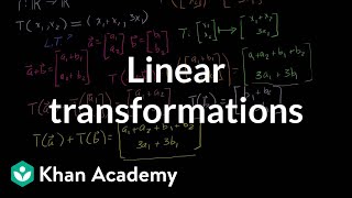
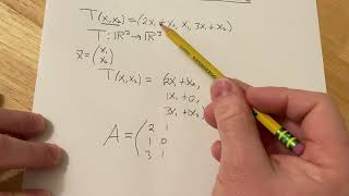
Youtube Videos


Audio Book
Dive deep into the subject with an immersive audiobook experience.
Definition of Linear Transformations
Chapter 1 of 3
🔒 Unlock Audio Chapter
Sign up and enroll to access the full audio experience
Chapter Content
A linear transformation (or linear map) between two vector spaces V and W over the same field 𝔽 is a function T: V → W such that for all u, v ∈ V and a ∈ 𝔽:
- T(u + v) = T(u) + T(v)
- T(a·v) = a·T(v)
Detailed Explanation
A linear transformation is a special type of function that takes vectors from one vector space (V) and transforms them into another vector space (W). For this function to be considered linear, it must satisfy two main properties:
1. Additivity: If you take two vectors u and v from the vector space V, the transformation of their sum (T(u + v)) must equal the sum of their individual transformations (T(u) + T(v)). This means the transformation preserves vector addition.
2. Homogeneity: If you take a vector v from V and multiply it by a scalar a from the field 𝔽, then transforming the scaled vector (T(a·v)) must equal the scalar multiplied by the transformation of the vector (a·T(v)). This means the transformation preserves scalar multiplication.
Examples & Analogies
Think of a linear transformation like a recipe for making a dish. If you double the ingredients (multiplying by a scalar), you expect to get twice the amount of food, just as a linear transformation doubles the transformed vector. Similarly, if you add two different ingredient portions together (adding vectors), the total amount of food must reflect the sum of those portions in the final dish. The recipe maintains the relationship between the ingredients in a straightforward manner, similar to how linear transformations maintain the relationships between vectors.
Important Properties of Linear Transformations
Chapter 2 of 3
🔒 Unlock Audio Chapter
Sign up and enroll to access the full audio experience
Chapter Content
- Important Properties:
- A linear transformation maps the zero vector in V to the zero vector in W:
T(0) = 0 - The image of a linear transformation is a subspace of W.
- The kernel (null space) of a linear transformation is a subspace of V.
Detailed Explanation
Linear transformations have specific properties that make them significant in vector spaces:
1. Zero Vector Mapping: A crucial aspect of linear transformations is that they send the zero vector (the vector with all components as zero) from the first vector space to the zero vector in the second vector space. This means that T(0) always equals 0. This property is essential because it ensures that the structure of the vector spaces is preserved.
2. Image is a Subspace: The set of all possible outputs (or images) of the linear transformation is called the image. This image forms a subspace of the target vector space W. This means that the image itself behaves like a vector space concerning vector addition and scalar multiplication.
3. Kernel is a Subspace: The kernel (or null space) consists of all vectors in V that map to the zero vector in W. This set also forms a subspace of V, indicating that the original vector space maintains its structure even while being transformed.
Examples & Analogies
Imagine a factory that processes raw materials into finished products. The raw materials represent the vectors in vector space V, and the finished products represent the vectors in vector space W. The linear transformation is akin to the manufacturing process. The zero material input (zero vector) produces no finished product (zero output). The finished products come together to form a new subset of items (the image) that also fits the definition of a product class. Furthermore, if some raw materials fail the quality check and become waste (kernel), they still constitute a specific group of unusable materials that forms an internal category within the factory's inventory.
Matrix Representation of Linear Transformations
Chapter 3 of 3
🔒 Unlock Audio Chapter
Sign up and enroll to access the full audio experience
Chapter Content
Matrix Representation:
If V and W are finite-dimensional with bases, any linear transformation T can be represented by a matrix A, such that T(x) = A·x. This is particularly useful in Civil Engineering for transforming coordinate systems, stress-strain relations, and more.
Detailed Explanation
When the vector spaces V and W are finite-dimensional, we can represent linear transformations using matrices. Each vector space has a basis, which is a set of vectors that can be combined to form all other vectors in that space. To apply the linear transformation T to a vector x, you can multiply the matrix A (which represents T) by the vector x. This multiplication results in a new vector that is the image of x under the transformation T. This matrix representation simplifies calculations and makes it easier to visualize the transformations, especially in applications like Civil Engineering, where coordinate systems are frequently changed and manipulated.
Examples & Analogies
Think of using a map to navigate a city. The map represents a matrix, while your current location and destination are vectors. When you multiply the map (matrix) by your starting position (vector), you determine how to get to your destination (resulting vector). In Civil Engineering, similar to using maps for navigating cities, matrices help in transforming complex structures and systems, facilitating accurate calculations and designs in projects like bridges or buildings.
Key Concepts
-
Linear Transformation: A function preserving vector operations between spaces.
-
Image: The outcome of a linear transformation comprising all mapped vectors.
-
Kernel: The set of inputs mapping to the zero vector in the output space.
Examples & Applications
A rotation of vectors in 2D space can serve as a linear transformation, where each vector is rotated by a fixed angle.
Scaling vectors by multiplying them with a scalar value is a simple example of a linear transformation done through matrix multiplication.
Memory Aids
Interactive tools to help you remember key concepts
Rhymes
Linear functions connect in ways, they shift and scale in many plays.
Stories
Imagine a magic box that spins and scales different shapes. No matter the form of the shape you put inside, the box outputs strictly what’s allowed!
Memory Tools
T.I.M.E. for linear transformations - Transform, Image, Multiply, and Examine.
Acronyms
L.I.N.E. stands for Linear Is a Nice Example.
Flash Cards
Glossary
- Linear Transformation
A function between two vector spaces that preserves vector addition and scalar multiplication.
- Image
The set of all vectors in the target vector space resulting from applying a linear transformation.
- Kernel
The set of vectors in the original vector space that map to the zero vector in the target vector space under a linear transformation.
- Matrix Representation
The expression of a linear transformation as a matrix, allowing for easier computation.
Reference links
Supplementary resources to enhance your learning experience.