
Momentum Flux Correction Factor
Enroll to start learning
You’ve not yet enrolled in this course. Please enroll for free to listen to audio lessons, classroom podcasts and take practice test.
Interactive Audio Lesson
Listen to a student-teacher conversation explaining the topic in a relatable way.
Introduction to Stress Tensors
🔒 Unlock Audio Lesson
Sign up and enroll to listen to this audio lesson

Today, we are diving into stress tensors. Remember, stress is defined as force per unit area. Can anyone tell me how many components make up a stress tensor?

Nine components, right?
That's correct, Student_1! The nine components include normal stresses and shear stresses. What's the difference between them?

Normal stresses come from pressure and viscosity, while shear stresses are purely due to viscosity.
Exactly! Think of it like this: normal stresses act perpendicular to the surface, and shear stresses act parallel to it. This is crucial when analyzing fluid surfaces.
Control Volumes
🔒 Unlock Audio Lesson
Sign up and enroll to listen to this audio lesson

Control volumes are essential for analyzing fluid mechanics problems. Can anyone describe what constitutes a control volume?

It’s the region in space where you analyze the fluid flow and forces acting on it!
Right! When we analyze a control volume, we need to consider both body forces, like gravity, and surface forces from stress tensors. Why is it important to identify these forces?

Because they affect how fluid moves and can significantly influence pressure distributions!
Great point! In fact, understanding how these forces interact helps us simplify problems and make calculations easier.
Momentum Flux and Correction Factor
🔒 Unlock Audio Lesson
Sign up and enroll to listen to this audio lesson
Let’s talk about momentum flux correction factors! Can anyone explain why we need them in real fluid flows?
Because the velocity distributions are often not uniform in real-life scenarios?
Precisely! So, if we calculate momentum flux using the average velocity without adjusting for this distribution, what could happen?
We might end up with inaccurate predictions of force and flow behavior!
Exactly! This is why applying a correction factor is crucial. It helps us translate average velocity data into a more accurate reflection of momentum flux.
Applications of Reynolds Transport Theorem
🔒 Unlock Audio Lesson
Sign up and enroll to listen to this audio lesson
The Reynolds transport theorem plays a significant role in momentum analysis. Can anyone summarize its purpose?
It helps relate the changes in momentum within a control volume to the forces acting on it?
Great summary! In essence, it allows us to compute net forces based on momentum flux. Why is this particularly useful in fluid mechanics?
Because it provides a systematic approach to analyze complex flows!
Exactly! When you apply it effectively, you can derive meaningful insights into how fluids behave under various conditions.
Final Considerations on Pressure and Forces
🔒 Unlock Audio Lesson
Sign up and enroll to listen to this audio lesson
To wrap up our session, let’s discuss pressures acting on control surfaces. Why do we often neglect atmospheric pressure in our calculations?
Because it acts equally in all directions, so it cancels out during surface integration?
Exactly! This simplification allows us to focus on gauge pressure and makes our calculations more manageable. What else can we exclude when calculating forces?
We might ignore effects when viscous forces aren't significant, right?
Spot on! Identifying simplifications leads to much clearer equations, allowing for more efficient problem-solving methods.
Introduction & Overview
Read summaries of the section's main ideas at different levels of detail.
Quick Overview
Standard
In this section, momentum flux correction factors are introduced to address the non-uniform velocity distributions in fluid flow systems. The concept of stress tensors is explored, detailing how they represent surface forces through their nine components. Emphasis is placed on normal and shear stress components, as well as the application of control volume principles and Reynolds transport theorem in fluid dynamics.
Detailed
Momentum Flux Correction Factor
In this section, we explore the momentum flux correction factor, a crucial concept in fluid mechanics. The correction factor accounts for the non-uniform velocity distributions that often occur in real-world fluid systems.
Key Concepts: Stress Tensors
- Stress Tensors: Stress is conceptualized as force per unit area, characterized by a stress tensor comprising nine components. These components include normal stresses (resulting from pressure and viscous forces) and shear stresses (due to viscosity). Understanding these forces is essential for analyzing fluid behavior and its effects on structures and systems.
- Control Volumes: The concept of control volumes is introduced, underscoring how surface and body forces interact within these volumes. The total force acting on a control volume is derived from both body forces (like gravity) and surface forces (influenced by stress tensors).
- Atmospheric Pressure: The section highlights that variables like atmospheric and gauge pressures are vital in defining pressure diagrams for control volumes, often allowing for the cancellation of atmospheric pressure in calculations.
- Application of Reynolds Transport Theorem: By utilizing the Reynolds transport theorem, the section examines how to articulate momentum equations and calculate net forces based on momentum flux.
Overall, this section elaborates on the pivotal role of momentum flux correction factors in ensuring accurate predictions of fluid behavior across various engineering applications.
Youtube Videos


Audio Book
Dive deep into the subject with an immersive audiobook experience.
Introduction to Momentum Flux Correction Factor
Chapter 1 of 4
🔒 Unlock Audio Chapter
Sign up and enroll to access the full audio experience
Chapter Content
Now, if you look it that way, now we can write the momentum equations in different forms considering the velocity distribution. That is the reason we introduce correction factors. That means, as we know it, the velocity distribution is not uniform for real fluid flow problems, computing this momentum flux using the average velocity, then what could be the correction factor for that.
Detailed Explanation
In fluid mechanics, the calculation of momentum flux is often done using the average velocity. However, in real fluid flows, the velocity is rarely uniform across the flow area. To make accurate calculations, we introduce a momentum flux correction factor, often denoted as beta (β). This factor adjusts for discrepancies in velocity distribution and ensures that our computations reflect the true conditions of the fluid flow.
Examples & Analogies
Think of it like measuring the average temperature in a room. If a heater is running in one corner, the temperature will vary throughout the room. If you only take one temperature reading (the average), you might miss hot and cold spots. The correction factor is like realizing you need to take readings in multiple places to get a true sense of the room's temperature.
Factors Affecting Momentum Flux
Chapter 2 of 4
🔒 Unlock Audio Chapter
Sign up and enroll to access the full audio experience
Chapter Content
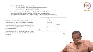
So, if you look at the velocity distribution, you can compute what will be the beta value for a velocity distribution coming into a cross section. Like, I have a pipe of laminar flow, a pipe of turbulent flow, or it is an open channel flow it is connecting, but each case we know approximate velocity distribution.
Detailed Explanation
The momentum flux correction factor is affected by the flow characteristics: laminar flow, turbulent flow, and open channel flow. Each of these flow types has a unique velocity distribution pattern. For instance, in laminar flow, fluid moves in layers, resulting in a parabolic velocity profile, whereas in turbulent flow, the velocity is more evenly distributed throughout. Knowing the flow type allows us to estimate the appropriate beta value to use in momentum calculations.
Examples & Analogies
Imagine a crowded highway. In smooth, laminar traffic, cars move in orderly lanes at consistent speeds. However, during rush hour, traffic becomes turbulent, with cars darting in and out of lanes. The consistent flow patterns in laminar flow can be effectively predicted, while chaotic, turbulent conditions require a different approach to understand overall flow dynamics.
Application of Momentum Flux Correction Factor
Chapter 3 of 4
🔒 Unlock Audio Chapter
Sign up and enroll to access the full audio experience
Chapter Content
This means, for each case we know what is the β value. If I know the β value, then we need do the integrations again. We use that beta value to convert from average velocity data to the momentum flux.
Detailed Explanation
Once the beta value is determined based on the velocity distribution, it is utilized in momentum equations to improve the accuracy of the momentum flux calculations. Effectively, the beta value allows us to convert our average velocity data into a more accurate representation of momentum flux by accounting for the variability of velocity across the flow area.
Examples & Analogies
Consider baking cookies. If a recipe says to cook at 350°F but your oven heats unevenly, using an average oven temperature won’t yield perfect cookies. If you know your oven is hotter in one corner (like knowing your velocity distribution), you may adjust the temperature for that section instead of sticking with the average, ensuring consistent baking results across your batch.
Summarizing Momentum Flux in Engineering
Chapter 4 of 4
🔒 Unlock Audio Chapter
Sign up and enroll to access the full audio experience
Chapter Content
Sum of the force acting on that will be equal to the net momentum flux passing through this control surface, that is what will come. So, let us have this for uniform flow. So, β will be equal to 1 and this thing if I do the integration of the velocities and the scalar products of V and n over a surface A, and that is what I am representing in average.
Detailed Explanation
In engineering contexts, the total force acting on a control volume is balanced by the net momentum flux that passes through its surfaces. When flow is uniform, the correction factor β equals 1, simplifying calculations as the average velocity directly approximates the actual momentum flux. Clarifying this balance is crucial to effective fluid mechanics applications.
Examples & Analogies
Think about measuring water flowing from a hose. If the flow is steady and consistent (uniform), you can easily calculate how much water comes out based on the average speed. But if the water starts to gush out wildly (non-uniform), you’ll need to account for those fluctuations (using a correction factor) to accurately gauge how much water you’re actually getting.
Key Concepts
-
Stress Tensors: Stress is conceptualized as force per unit area, characterized by a stress tensor comprising nine components. These components include normal stresses (resulting from pressure and viscous forces) and shear stresses (due to viscosity). Understanding these forces is essential for analyzing fluid behavior and its effects on structures and systems.
-
Control Volumes: The concept of control volumes is introduced, underscoring how surface and body forces interact within these volumes. The total force acting on a control volume is derived from both body forces (like gravity) and surface forces (influenced by stress tensors).
-
Atmospheric Pressure: The section highlights that variables like atmospheric and gauge pressures are vital in defining pressure diagrams for control volumes, often allowing for the cancellation of atmospheric pressure in calculations.
-
Application of Reynolds Transport Theorem: By utilizing the Reynolds transport theorem, the section examines how to articulate momentum equations and calculate net forces based on momentum flux.
-
Overall, this section elaborates on the pivotal role of momentum flux correction factors in ensuring accurate predictions of fluid behavior across various engineering applications.
Examples & Applications
Example 1: In a cylindrical pipe with laminar flow, the velocity distribution shows highest velocity at the center. This necessitates the use of a momentum flux correction factor when calculating momentum flux using average velocity.
Example 2: Considering a free jet impacting a surface, the momentum flux is influenced by the non-uniform velocity profile, which, again, calls for an appropriate adjustment using a momentum flux correction factor.
Memory Aids
Interactive tools to help you remember key concepts
Rhymes
A tensor's shape is a square, forces within it, we declare!
Stories
Imagine a fluid dancing in a pipe, it swirls and turns with a speedy type; at the center it's rushing, while at the side it's slow, knowing this, a correction factor we'll bestow!
Memory Tools
Remember: 'Tensile sharp, shear as a dart'—a stress tensor brings force apart!
Acronyms
S.N.S
Stresses
Normal
and Shear—key components we must hold near!
Flash Cards
Glossary
- Stress Tensor
A mathematical representation describing the distribution of internal forces within a material, typically expressed in a 3x3 matrix format representing nine components.
- Normal Stress
The stress component that acts perpendicular to a surface, resulting from pressure and viscous forces.
- Shear Stress
The stress component that acts parallel to a surface, primarily due to viscosity.
- Control Volume
A fixed region in space used for analyzing fluid flow and force interactions.
- Momentum Flux Correction Factor
A numeric factor used to adjust the average velocity in momentum calculations to account for non-uniform velocity distributions.
Reference links
Supplementary resources to enhance your learning experience.