
Extended Example: 3×3 Matrix
Enroll to start learning
You’ve not yet enrolled in this course. Please enroll for free to listen to audio lessons, classroom podcasts and take practice test.
Interactive Audio Lesson
Listen to a student-teacher conversation explaining the topic in a relatable way.
Finding the Characteristic Polynomial
🔒 Unlock Audio Lesson
Sign up and enroll to listen to this audio lesson

Today we will explore how to find the characteristic polynomial of a 3×3 matrix. Can anyone remind us why we need it?

It's used to find the eigenvalues!
Exactly! The characteristic polynomial is calculated by finding the determinant of the matrix minus lambda times the identity matrix, denoted as det(A - λI). Let's apply this with our matrix A.

What matrix are we using?
Let’s use $$ A = \begin{bmatrix} 2 & 0 & 0 \\\ 0 & 3 & 4 \\\ 0 & 4 & 3 \end{bmatrix} $$ and compute det(A - λI). What would that look like?

We plug λ into the diagonal, right? So we'll have (2-λ) in the first row.
That's correct! Let’s expand it step-by-step together.
Deriving Eigenvalues
🔒 Unlock Audio Lesson
Sign up and enroll to listen to this audio lesson

After calculating the determinant, we set it equal to zero to find the eigenvalues. What do we call the values we find?
Eigenvalues!
Correct! So after finding the characteristic polynomial, we derived that eigenvalues are λ = 2, 7, and -1. Can someone elaborate why these are so important?

They help us understand the behavior of the system represented by the matrix, such as its stability.
Spot on! Now, let’s discuss how we can find the respective eigenvectors for these eigenvalues.
Finding Eigenvectors
🔒 Unlock Audio Lesson
Sign up and enroll to listen to this audio lesson
Now that we have our eigenvalues, let’s find the eigenvector for λ = 2. We solve (A - 2I)v = 0. Can anyone share what this means?
It means we are effectively solving a homogeneous system.
Exactly! As we simplify, we should look for linearly independent solutions. How do we find those from our row-reduced matrix?
We can express one variable in terms of another and find the relationships!
Right! And for λ = 2, we will find the eigenvector is $$ v = \begin{bmatrix} 1 \\\ 0 \\\ 0 \end{bmatrix} $$. Fantastic work, everyone!
Application and Significance of Eigenvalues and Eigenvectors
🔒 Unlock Audio Lesson
Sign up and enroll to listen to this audio lesson
Lastly, how do eigenvalues and eigenvectors apply in engineering, specifically in structural analysis?
They help in analyzing dynamic responses of structures to loads and vibrations.
Great! This application underscores how the study of matrices can shape our understanding of engineering systems.
Are there cases when eigenvectors can't be found easily?
Good question! Sometimes, eigenvectors may not be real or may be difficult to compute. This often calls for complex analysis.
What about degenerate eigenvalues?
In such cases, multiple independent eigenvectors may exist, and careful handling is necessary. Excellent conversation today!
Introduction & Overview
Read summaries of the section's main ideas at different levels of detail.
Quick Overview
Standard
In this section, we examine a specific 3x3 matrix, detailing the steps required to derive its eigenvalues by evaluating the characteristic polynomial, and subsequently finding the corresponding eigenvectors. This example illustrates the application of theoretical concepts in practical scenarios, essential for understanding matrix behavior.
Detailed
Detailed Summary
In this section, we explore an extended example using a 3×3 matrix to illustrate the process of finding eigenvalues and eigenvectors. We start with the matrix:
$$
A = \begin{bmatrix} 2 & 0 & 0 \\ 0 & 3 & 4 \\ 0 & 4 & 3 \end{bmatrix}
$$
Step 1: Characteristic Polynomial
The characteristic polynomial is derived from the determinant of the matrix $(A - \lambda I)$, which is calculated as:
$$
\text{det}(A - \lambda I) = \text{det} \begin{bmatrix} 2-\lambda & 0 & 0 \\ 0 & 3-\lambda & 4 \\ 0 & 4 & 3-\lambda \end{bmatrix}.
$$
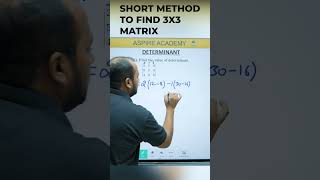
By expanding this determinant, we get:
$$
(2 - \lambda)((3 - \lambda)(3 - \lambda) - 16) = (2 - \lambda)(7 - \lambda)(-1 - \lambda).
$$
Thus, the eigenvalues are:
- $\lambda_1 = 2$
- $\lambda_2 = 7$
- $\lambda_3 = -1$
Step 2: Find Eigenvectors
Next, we determine the corresponding eigenvectors for each eigenvalue:
- For $\lambda = 2$:
$$
(A - 2I)v = 0\Rightarrow \begin{bmatrix} 0 & 0 & 0 \\ 0 & 1 & 4 \\ 0 & 4 & 1 \end{bmatrix} \begin{bmatrix} v_1 \\ v_2 \\ v_3 \end{bmatrix} = \begin{bmatrix} 0 \\ 0 \\ 0 \end{bmatrix}.
$$
Solving yields the eigenvector corresponding to $\lambda = 2$ as:
$$
v = \begin{bmatrix} 1 \\ 0 \\ 0 \end{bmatrix}.
$$
- For $\lambda = 7$ and $\lambda = -1$, similar computations yield their respective eigenvectors.
This practical numeral example emphasizes the process of finding eigenvalues and eigenvectors, which ultimately contributes to applications in structural engineering and other fields. By placing focus on direct calculations, students gain better comprehension of how theoretical concepts are put into practice.
Youtube Videos


Audio Book
Dive deep into the subject with an immersive audiobook experience.
Step 1: Characteristic Polynomial
Chapter 1 of 3
🔒 Unlock Audio Chapter
Sign up and enroll to access the full audio experience
Chapter Content
Let us consider the matrix:
\[ A = \begin{bmatrix} 2 & 0 & 0 \\ 0 & 3 & 4 \\ 0 & 4 & 3 \end{bmatrix} \]
Step 1: Characteristic Polynomial
\[ det(A-\lambda I)=det \begin{bmatrix} 2-\lambda & 0 & 0 \\ 0 & 3-\lambda & 4 \\ 0 & 4 & 3-\lambda \end{bmatrix} \]
Expanding along the first row:
\[ (2-\lambda) \cdot det \begin{bmatrix} 3-\lambda & 4 \\ 4 & 3-\lambda \end{bmatrix} \]
So, eigenvalues are:
\[ \lambda = 2, \lambda = 7, \lambda = -1 \]
Detailed Explanation
In this step, we start with a 3x3 matrix and seek to find its characteristic polynomial. The characteristic polynomial is obtained by subtracting an eigenvalue (represented as λ) multiplied by the identity matrix I from our original matrix A and calculating the determinant of the resulting matrix. This determinant is set to zero to find the eigenvalues. In this case, we find that our eigenvalues are λ = 2, λ = 7, and λ = -1.
Examples & Analogies
Think of the characteristic polynomial like a recipe where the ingredients (our matrix A and λ) must blend perfectly to create the dish (which in this case is the behavior of the matrix determined by its eigenvalues). When we find the perfect mix and set our recipe (the determinant) to zero, we uncover the tasty secrets (eigenvalues) that our matrix holds.
Step 2: Finding Eigenvectors
Chapter 2 of 3
🔒 Unlock Audio Chapter
Sign up and enroll to access the full audio experience
Chapter Content
Step 2: Find Eigenvectors
For \( \lambda=2:\n \[ A - 2I = \begin{bmatrix} 0 & 0 & 0 \\ 0 & 1 & 4 \\ 0 & 4 & 1 \end{bmatrix} \]
Solve:
\[ (A-2I)v=0 \]
This implies: \[ v_1 = 0, v_2 = 0, v_3 = free \Rightarrow v = \begin{bmatrix} 1 \\ 0 \\ 0 \end{bmatrix} \]
Thus, basis of eigenvectors for \( \lambda=2: \{\begin{bmatrix} 1 \ 0 \ 0 \end{bmatrix}\}
Detailed Explanation
After identifying the eigenvalue λ = 2, we proceed to find the corresponding eigenvector. This involves substituting λ back into the modified matrix (A - 2I) and then solving the resulting system of equations for the vector v. The solution provides us with the basis for eigenvectors related to this eigenvalue. Here, we find that the eigenvector for λ = 2 is simply [1, 0, 0], which indicates a direction in our vector space.
Examples & Analogies
Finding eigenvectors can be compared to determining the specific route to take when navigating a city. Just like there are multiple roads leading to your destination, each eigenvalue provides a unique direction (or eigenvector) that exhibits how the matrix will behave. When the eigenvalue is 2, this particular route corresponds simply to one straight road marked as [1, 0, 0].
Eigenvectors for Other Eigenvalues
Chapter 3 of 3
🔒 Unlock Audio Chapter
Sign up and enroll to access the full audio experience
Chapter Content
Similarly solve for \( \lambda=7 \) and \( \lambda=-1 \):
Detailed Explanation
In this part of the exercise, we apply the same method to determine the eigenvectors associated with the remaining eigenvalues, λ = 7 and λ = -1. By updating our calculations based on these eigenvalues and solving the equations formed from (A - λI)v = 0, we will find specific directions (eigenvectors) for each eigenvalue. Although the specific calculations are not shown here, they follow the pattern established in finding the eigenvector for λ = 2.
Examples & Analogies
Imagine you are exploring different paths in a park. Each path represents an eigenvalue leading you through different sections of the park. Just like you would take time to explore each path based on the unique scenery it offers, we explore each eigenvalue to uncover its unique eigenvectors, understanding how they each contribute to the overall layout (or behavior) of the park (or matrix).
Key Concepts
-
Characteristic Polynomial: A polynomial representation that helps find eigenvalues.
-
Eigenvalues: The scalars that determine the factor by which a corresponding eigenvector is scaled.
-
Eigenvectors: Vectors that indicate direction along which a transformation acts by stretching or compressing.
-
Eigenspace: The subspace spanned by one or more eigenvectors, corresponding to an eigenvalue.
Examples & Applications
A 3x3 matrix A is given. By finding the characteristic polynomial and its roots, we derive eigenvalues of λ = 2, 7, -1, and subsequently find corresponding eigenvectors.
Memory Aids
Interactive tools to help you remember key concepts
Rhymes
Eigenvalues are like stars in the night, they shine bright, showing matrix's might.
Stories
Imagine a magician named Eigen who could only stretch or shrink objects but never change their direction. That’s what an eigenvector does!
Memory Tools
To find eigenvalues: Derive, Set, Solve! (Derive characteristic polynomial, set to zero, solve for λ.)
Acronyms
EVE
Eigenvalue
Vector
Eigenspace.
Flash Cards
Glossary
- Characteristic Polynomial
A polynomial derived from the matrix that is used to find eigenvalues.
- Eigenvalue
A scalar λ such that there exists a non-zero vector v satisfying Av = λv.
- Eigenvector
A non-zero vector v associated with an eigenvalue λ.
- Eigenspace
The set of all eigenvectors corresponding to a given eigenvalue, including the zero vector.
Reference links
Supplementary resources to enhance your learning experience.