
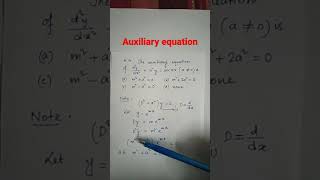
Auxiliary Equation (AE)
Enroll to start learning
You’ve not yet enrolled in this course. Please enroll for free to listen to audio lessons, classroom podcasts and take practice test.
Interactive Audio Lesson
Listen to a student-teacher conversation explaining the topic in a relatable way.
Introduction to Auxiliary Equation
🔒 Unlock Audio Lesson
Sign up and enroll to listen to this audio lesson

Today, we'll discuss the Auxiliary Equation, which helps us solve homogeneous linear differential equations with constant coefficients. Can someone tell me what a second-order linear differential equation looks like?

Isn't it something like d²y/dx² + b(dy/dx) + cy = 0?
Exactly! To solve it, we derive the Auxiliary Equation, which is am² + bm + c = 0. This quadratic equation gives us valuable information about the roots, which leads us to the general solution.

What do we do with those roots?
Good question! Depending on whether the roots are real and distinct, real and equal, or complex, we'll have different forms of the solution.

Can you remind us how to classify the roots?
Sure! We use the discriminant from the quadratic formula: if it’s positive, we get real and distinct roots; if zero, real and equal roots; and if negative, complex roots.
So, let me summarize: The Auxiliary Equation is crucial for finding the roots of a differential equation, and knowing these roots allows us to write the general solution.
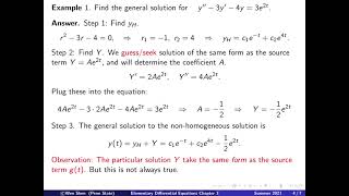
Case I – Real and Distinct Roots
🔒 Unlock Audio Lesson
Sign up and enroll to listen to this audio lesson

Let's dive into Case I where we have real and distinct roots. What does that mean for our general solution?

I think it means we can write the general solution as y = C₁e^(m₁x) + C₂e^(m₂x).
Exactly! Here, 'C₁' and 'C₂' are constants that we determine based on initial conditions. Why do you think this form is useful in applications?
Because it represents the superposition of two different exponential behaviors, which is common in physical systems.
Correct! This flexibility allows engineers to model various phenomena in civil engineering effectively.
To wrap up, Case I's real and distinct roots give us a clear path for forming the solution using two exponential terms.
Case II – Real and Equal Roots
🔒 Unlock Audio Lesson
Sign up and enroll to listen to this audio lesson
Now, who can tell me about Case II with real and equal roots?
That's when we get a repeated root, right? The solution is y = (C₁ + C₂x)e^(mx)?
Yes! The introduction of 'x' allows us to account for the multiplicity of the root. Why might repeated roots occur in real-world problems?
It might represent a system approaching a steady state, like a damped oscillator reaching equilibrium.
Spot on! This case shows how we can capture complex dynamics using the Auxiliary Equation. Let’s summarize: Real and equal roots lead us to a solution that incorporates a linear factor.
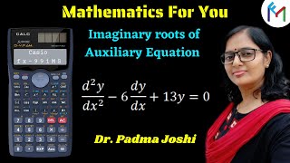
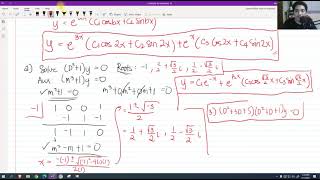
Case III – Complex Roots
🔒 Unlock Audio Lesson
Sign up and enroll to listen to this audio lesson
Finally, let's talk about Case III where we have complex roots. What does that formula look like?
It’s y = e^(αx)(C₁cos(βx) + C₂sin(βx)).
Precisely! This allows us to express oscillatory behavior, very common in engineering systems. How can we visualize this behavior?
We can think of it like waves, where the e^(αx) factor represents exponential growth or decay, and the sine and cosine functions represent oscillation.
That's an excellent visualization! Remember, this solution structure helps us model phenomena like vibrations in beams or electrical circuits.
To summarize, complex roots lead us to a solution that captures oscillatory behavior, essential in many engineering applications.
Introduction & Overview
Read summaries of the section's main ideas at different levels of detail.
Quick Overview
Standard
In this section, we explore the concept of the Auxiliary Equation (AE) derived from homogeneous linear differential equations with constant coefficients. We identify three main cases based on the nature of the roots—real and distinct, real and equal, and complex—and their respective general solution forms.
Detailed
Auxiliary Equation (AE)
The Auxiliary Equation is a crucial tool in solving homogeneous linear differential equations that have constant coefficients. In a general form of second-order linear differential equations:
d²y/dx² + b(dy/dx) + cy = 0,
where 'a', 'b', and 'c' are constants, we set the Auxiliary Equation as:
am² + bm + c = 0
This quadratic polynomial can be solved to find the roots 'm₁' and 'm₂'. The classification of these roots determines the general solution of the differential equation:
- Case I: Real and Distinct Roots (m₁, m₂)
-
General solution:
y = C₁e^(m₁x) + C₂e^(m₂x)
where 'C₁' and 'C₂' are constants. - Case II: Real and Equal Roots (m)
-
General solution:
y = (C₁ + C₂x)e^(mx) - Case III: Complex Roots (α ± iβ)
- General solution:
y = e^(αx)(C₁cos(βx) + C₂sin(βx))
Each case showcases the diverse behaviors of solutions to linear differential equations, illustrating the complexity that arises in engineering applications.
Youtube Videos


![Mathematics| ODE |Linear Differential Equations With constant coefficients [Repeated roots of A.E.]](https://img.youtube.com/vi/KnVdG4YnLqg/mqdefault.jpg)


Audio Book
Dive deep into the subject with an immersive audiobook experience.
Definition of the Auxiliary Equation
Chapter 1 of 5
🔒 Unlock Audio Chapter
Sign up and enroll to access the full audio experience
Chapter Content
The Auxiliary Equation (AE) is given by the formula:
am^2 + b m + c = 0
Detailed Explanation
The Auxiliary Equation is a characteristic polynomial formed from a linear differential equation with constant coefficients. Here, 'a', 'b', and 'c' are constants derived from the original differential equation, while 'm' represents the roots of this polynomial. Finding the roots of the Auxiliary Equation helps us determine the general solution of the associated differential equation.
Examples & Analogies
Think of the Auxiliary Equation like the recipe for a dish. Just as specific ingredients lead to a particular flavor, the constants 'a', 'b', and 'c' in the Auxiliary Equation lead to specific 'flavors' of solutions for the differential equation.
Solving the Auxiliary Equation
Chapter 2 of 5
🔒 Unlock Audio Chapter
Sign up and enroll to access the full audio experience
Chapter Content
We solve for roots m1, m2 and classify them into three cases:
1. Case I: Real and distinct roots m1, m2
2. Case II: Real and equal roots m
3. Case III: Complex roots m = α ± iβ
Detailed Explanation
When we solve the Auxiliary Equation, we find two types of roots that determine the form of the general solution to the differential equation. In Case I, if the roots are real and distinct, the solution combines exponential functions. In Case II, when the roots are equal, a linear term multiplied by an exponential function appears. In Case III, where the roots are complex, we see oscillatory behavior represented by sine and cosine functions coupled with exponentials.
Examples & Analogies
Consider each case like different paths to reach a destination by bus. Case I, with different routes (real and distinct), allows you to take different buses (representing exponential functions). Case II is like having one bus that makes multiple stops (equal roots), while Case III is like a scenic route where you encounter both hills and valleys (complex roots) with ups and downs.
Case I: Real and Distinct Roots
Chapter 3 of 5
🔒 Unlock Audio Chapter
Sign up and enroll to access the full audio experience
Chapter Content
For real and distinct roots m1, m2:
y = C1 e^(m1 x) + C2 e^(m2 x)
Detailed Explanation
When we find two different real roots, 'm1' and 'm2', the general solution takes the form of a sum of exponential functions. The constants 'C1' and 'C2' are determined by the initial conditions of the problem, allowing us to tailor the solution to specific scenarios.
Examples & Analogies
Imagine planting two different types of trees in a garden (the roots). Each tree grows in its own unique way as it gets sunlight and water (the exponential functions). The combination of both trees growing together represents the complete solution to our differential equation.
Case II: Real and Equal Roots
Chapter 4 of 5
🔒 Unlock Audio Chapter
Sign up and enroll to access the full audio experience
Chapter Content
For real and equal roots m:
y = (C1 + C2 x)e^(m x)
Detailed Explanation
In cases where both roots are the same, the general solution must include a term that accounts for the 'multiplicity' of that root. This results in an extra 'x' factor multiplying one of the constants, leading to a modified exponential form. This situation often leads to solutions that grow more quickly than those with distinct roots due to the presence of this linearity.
Examples & Analogies
Think about a competition where the same athlete wins multiple times (equal roots). Their consistently strong performance leads to even greater visibility and growth in popularity (the solution's growth is accelerated). Thus, we need an expression that reflects not just the winning but the context in which it happens.
Case III: Complex Roots
Chapter 5 of 5
🔒 Unlock Audio Chapter
Sign up and enroll to access the full audio experience
Chapter Content
For complex roots m = α ± iβ:
y = e^(α x)(C1 cos(β x) + C2 sin(β x))
Detailed Explanation
Complex roots introduce oscillatory behavior in the solution due to the sine and cosine terms. The real part, 'α', leads to exponential growth or decay, while the imaginary part, 'β', represents oscillations. This results in behavior that can be periodic, a common feature in many engineering applications encountered in vibrations or waves.
Examples & Analogies
Picture a pendulum swinging back and forth -- the oscillation (the sine and cosine) combined with a gradual slowing down as it loses energy (the exponential decay related to 'α'). Here, the complex roots illustrate both the rhythm of swinging and the underlying energy loss.
Key Concepts
-
Auxiliary Equation: A quadratic equation used to determine the roots for solving differential equations.
-
Real and Distinct Roots: Separate root values leading to a solution that encompasses two exponentials.
-
Real and Equal Roots: A repeated root resulting in a solution that includes a linear factor with an exponential.
-
Complex Roots: Roots that result in oscillatory solutions combining exponential decay and sine/cosine terms.
Examples & Applications
For the equation d²y/dx² - 5(dy/dx) + 6y = 0, the Auxiliary Equation is m² - 5m + 6 = 0, yielding roots m₁ = 2 and m₂ = 3, leading to the general solution y = C₁e^(2x) + C₂e^(3x).
For the equation d²y/dx² - 4y = 0, the Auxiliary Equation m² - 4 = 0 yields roots m₁ = ±2, leading to a solution of y = C₁e^(2x) + C₂e^(-2x) for real and distinct roots.
Memory Aids
Interactive tools to help you remember key concepts
Rhymes
Roots of the AE, they must relate,
Stories
Once upon a time, there was an engineer named Al who was tasked with solving differential equations. One day he discovered an Auxiliary Equation that helped him find roots, leading to distinct exponential solutions that were essential for his bridge design—he became known as the Wizard of Waves in the world of engineering!
Memory Tools
R.E.C. can help you recall the types of roots: Real and Distinct, Real and Equal, and Complex!
Acronyms
Remember the acronym 'R.E.C.'
for Real and Distinct
for Equal
for Complex in roots of the Auxiliary Equation!
Flash Cards
Glossary
- Auxiliary Equation
A quadratic equation derived from a second-order linear differential equation, used to find the roots necessary to construct the general solution.
- Real and Distinct Roots
Two different real numbers that satisfy the Auxiliary Equation, leading to a general solution of the form y = C₁e^(m₁x) + C₂e^(m₂x).
- Real and Equal Roots
A single real number that is repeated as a root, leading to a general solution of the form y = (C₁ + C₂x)e^(mx).
- Complex Roots
Roots of the Auxiliary Equation that are complex numbers, leading to a general solution of the form y = e^(αx)(C₁cos(βx) + C₂sin(βx)).
Reference links
Supplementary resources to enhance your learning experience.