
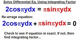
Solution Method: Integrating Factor (IF)
Enroll to start learning
You’ve not yet enrolled in this course. Please enroll for free to listen to audio lessons, classroom podcasts and take practice test.
Interactive Audio Lesson
Listen to a student-teacher conversation explaining the topic in a relatable way.
Understanding the Integrating Factor
🔒 Unlock Audio Lesson
Sign up and enroll to listen to this audio lesson

Today, we will explore a powerful method called the Integrating Factor for solving first-order linear differential equations. Can anyone tell me what a first-order linear DE looks like?

I think it has the form dy/dx + P(x)y = Q(x).
Exactly! Now, the key to solving these equations lies in calculating an Integrating Factor. We denote it as μ(x). Does anyone know how we find this factor?

Isn't it e raised to the integral of P(x) dx?
Right again! So, we compute μ(x) using that formula. This will help us transform the equation. Let's move on to how it transforms the equation. Remember the acronym MPE—Multiply, Transform, and Integrate.
Transforming the Equation with the Integrating Factor
🔒 Unlock Audio Lesson
Sign up and enroll to listen to this audio lesson

After calculating the Integrating Factor, we multiply the entire differential equation by μ(x). What does this do?

It makes the left side an exact derivative, right?
Correct! We end up with d/dx[μ(x)y] = μ(x)Q(x). This shows that the left side is the derivative of the product, which simplifies our work. What comes next after we get this form?

We integrate both sides, I believe.
Exactly! Let's summarize: first, we calculate μ(x), we multiply, transform, and finally integrate. Remember, MPE helps keep these steps in mind.
Integrating the Equation
🔒 Unlock Audio Lesson
Sign up and enroll to listen to this audio lesson
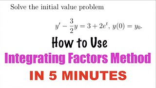
Let's take an example: solve dy/dx + 2y = e^(-x). What should we do first?
First, we identify P(x) which is 2. Then, we find μ(x).
Correct! So, computing μ(x) gives us e^(2x). What do we do next?
We multiply the equation by e^(2x).
Exactly! After that, rewrite it as d/dx[e^(2x)y] = e^(-x)e^(2x). Now what?
We integrate both sides!
Great! After integrating, we can determine our general solution. It’s essential to practice these steps for mastery.
Final Steps and Applications
🔒 Unlock Audio Lesson
Sign up and enroll to listen to this audio lesson
Now that we have our general solution, how can we evaluate it further?
If we have specific initial conditions, we can find C, the constant.
Exactly! Knowing how to solve and then apply these solutions is crucial in engineering contexts. Can anyone think of a situation where this might apply?
In systems that model heat transfer, like conduction in concrete?
Spot on! Integrating Factors are indeed vital in applications like those. Let's review: we found μ(x), transformed the equation, integrated, and applied our solutions. Keep practicing!
Introduction & Overview
Read summaries of the section's main ideas at different levels of detail.
Quick Overview
Standard
In this section, the Integrating Factor (IF) method is detailed as a systematic approach to solve first-order linear differential equations. It involves multiplying the equation by an integrating factor derived from the coefficient of the dependent variable, simplifying the equation into an exact differential, allowing for straightforward integration.
Detailed
Solution Method: Integrating Factor (IF)
The Integrating Factor method is a primary technique used in solving first-order linear differential equations of the form:
\[ \frac{dy}{dx} + P(x)y = Q(x) \]
Where \( P(x) \) and \( Q(x) \) are continuous functions of \( x \). The solution process involves three significant steps:
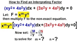
- Multiply both sides by the Integrating Factor:
- The Integrating Factor, \( \mu(x) \), is calculated as:
\[ \mu(x) = e^{\int P(x) \, dx} \] - This transformation allows the left side of the equation to become an exact derivative of the product \( \mu(x)y \).
- Rewrite the equation:
-
The equation is then expressed in the form:
\[ \frac{d}{dx}[\mu(x)y] = \mu(x)Q(x) \] - Integrate both sides:
- Upon integrating both sides, you get:
\[ y = \frac{1}{\mu(x)}\int \mu(x)Q(x) \, dx + C \] - \( C \) is the constant of integration, determined from initial conditions or boundary values.
This method efficiently converts a linear differential equation into a solvable integral form, highlighting its application and utility in various engineering contexts.
Youtube Videos


Audio Book
Dive deep into the subject with an immersive audiobook experience.
Integrating Factor Definition
Chapter 1 of 4
🔒 Unlock Audio Chapter
Sign up and enroll to access the full audio experience
Chapter Content
The standard method to solve is:
1. Multiply both sides by an integrating factor:
R \[
\mu(x)=e^{\int P(x)dx}
\]
2. This transforms the equation into:
\[
\frac{d}{dx}[\mu(x)y]=\mu(x)Q(x)
\]
3. Integrate both sides:
\[
y = \frac{\int \mu(x)Q(x)dx + C}{\mu(x)}
\]
Detailed Explanation
The integrating factor method is a powerful technique for solving first-order linear differential equations. The first step involves identifying the integrating factor, which is expressed as \( \mu(x) = e^{\int P(x)dx} \). This factor is then multiplied by both sides of the differential equation, effectively simplifying the equation. The transformation turns the standard first-order linear DE into an equation that can be integrated directly. After multiplying through by \( \mu(x) \), the left-hand side now represents the derivative of the product \( \mu(x)y \). The integral of the right-hand side gives us a function that we can then solve for \( y \), yielding the general solution of the differential equation.
Examples & Analogies
Think of the integrating factor like a special tool in a toolbox. Just as you might use a wrench to make it easier to tighten a bolt, multiplying the original equation by the integrating factor makes it easier to solve the differential equation. Once you have that tool (the integrating factor), you can ‘tighten’ the solution by integrating and finding the answer.
Multiplying by the Integrating Factor
Chapter 2 of 4
🔒 Unlock Audio Chapter
Sign up and enroll to access the full audio experience
Chapter Content
- Multiply both sides by an integrating factor:
R \[
\mu(x)=e^{\int P(x)dx}
\]
Detailed Explanation
To begin solving the first-order linear differential equation, we first calculate the integrating factor \( \mu(x) \). This factor is based on the function \( P(x) \) appearing in the equation. By taking the exponential of the integral of \( P(x) \), we create a multiplier that will facilitate the rewrite of our differential equation. This step is crucial because it transforms the equation into a form where the left-hand side can be expressed as the derivative of a product, specifically the product of \( \mu(x) \) and \( y \).
Examples & Analogies
Imagine if you're trying to solve a puzzle but find it difficult because some pieces just don’t fit well. By calculating the integrating factor, you’re essentially cleaning the puzzle pieces so they fit together nicely. Once the pieces fit together, the overall picture becomes clearer, allowing you to solve the puzzle more easily.
Transforming the Equation
Chapter 3 of 4
🔒 Unlock Audio Chapter
Sign up and enroll to access the full audio experience
Chapter Content
- This transforms the equation into:
\[
\frac{d}{dx}[\mu(x)y]=\mu(x)Q(x)
\]
Detailed Explanation
After multiplying both sides of the original differential equation by the integrating factor, the equation takes on a new form: \( \frac{d}{dx}[\mu(x)y]=\mu(x)Q(x) \). This transformation is critical because it consolidates the left-hand side into a single derivative. It signifies that the rate of change of the product \( \mu(x)y \) equals a modified version of \( Q(x) \), allowing us to utilize integration effectively. This step simplifies the overall problem into manageable parts.
Examples & Analogies
Think of this transformation like rearranging furniture in a room. By moving things around (like multiplying by the integrating factor), you create more space and clarity, making it easier to navigate through the room. The new arrangement (the transformed equation) reveals how everything interacts and allows you to see the solution more clearly.
Integrating Both Sides
Chapter 4 of 4
🔒 Unlock Audio Chapter
Sign up and enroll to access the full audio experience
Chapter Content
- Integrate both sides:
\[
y = \frac{\int \mu(x)Q(x)dx + C}{\mu(x)}
\]
Detailed Explanation
The final step in using the integrating factor method is integrating both sides of the transformed equation. This integration will yield a solution for \( y \) in terms of \( \mu(x) \) and an arbitrary constant \( C \). Integrating the right side with respect to \( x \) allows us to find the explicit function of \( y \). Hence, we end up with a general solution, which combines both the particular solution from \( Q(x) \) and the constant of integration.
Examples & Analogies
This process of integration is akin to finishing a recipe. You’ve gathered your ingredients (the equation) and mixed them (performed the transformations), and now it’s time to cook (integrate). Once you cook everything together, you reveal the final dish (the solution) that represents the relationship defined by the original equation.
Key Concepts
-
Integrating Factor: A function that modifies the original differential equation to enable easier integration.
-
Transformation of Differential Equations: The process by which the left side of an equation is transformed into an exact derivative.
-
General Solution: The solution of a differential equation including the constant of integration.
Examples & Applications
Example: For the equation dy/dx + 2y = e^(-x), the integrating factor is e^(2x), leading to the solution y = e^(-x) + Ce^(-2x).
Memory Aids
Interactive tools to help you remember key concepts
Rhymes
Integrate with glee, the factors of P; Multiply, transform, then set your y free.
Stories
Once there was a function struggling with derivatives. The Integrating Factor came to rescue, multiplying and transforming the equation to reveal secrets hidden in its form.
Memory Tools
MPE - Multiply (by μ), Transform (to an exact), Integrate (both sides).
Acronyms
IF = Integrating Factor. Remember
It's crucial in making equations integrable.
Flash Cards
Glossary
- Integrating Factor
A function used to multiply a differential equation to facilitate its integration.
- Firstorder linear differential equation
A differential equation involving only the first derivative of the dependent variable.
- Exact derivative
A derivative that can be expressed in the form of a single variable's derivative.
Reference links
Supplementary resources to enhance your learning experience.