
Homogeneous Equations with Constant Coefficients
Enroll to start learning
You’ve not yet enrolled in this course. Please enroll for free to listen to audio lessons, classroom podcasts and take practice test.
Interactive Audio Lesson
Listen to a student-teacher conversation explaining the topic in a relatable way.
General Form of Homogeneous Equations
🔒 Unlock Audio Lesson
Sign up and enroll to listen to this audio lesson

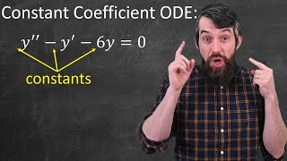
Today we are discussing homogeneous linear differential equations with constant coefficients. The general form is expressed as a second-order differential equation, given by a d²y/dx² + b dy/dx + cy = 0. Can anyone tell me what each term represents?

I think 'a', 'b', and 'c' are constants. And y is the dependent variable?
Correct! 'a', 'b', and 'c' are indeed constants that determine the behavior of the equation. The function y depends on the variable x. What does the term 'homogeneous' imply about our equation?

It means there are no external forces acting on the system, right?
Exactly! Now remember this with the acronym 'HEE'—Homogeneous equations have no external force. Let's move on to the Auxiliary Equation.
Auxiliary Equation
🔒 Unlock Audio Lesson
Sign up and enroll to listen to this audio lesson

The Auxiliary Equation or AE is derived from the homogeneous equation. It takes the form am² + bm + c = 0. Why do we use it?

Is it to find the roots that help us solve the differential equation?
Yes! By solving for the roots m, we identify the nature of the solutions. Could someone recap the result of finding the roots?

If we find real and distinct roots, we get exponential solutions; if they are equal, we add a linear term multiplied by the exponential; and with complex roots, we have oscillatory solutions.
Great summary! Remember: 'Roots Shape Solutions'—the type of roots informs the form of our solutions. Now, let's consider each case individually.
Cases of Roots
🔒 Unlock Audio Lesson
Sign up and enroll to listen to this audio lesson
Let’s discuss the three cases we derived from the Auxiliary Equation. The first is for real and distinct roots. What does the general solution look like?
It’s y = C₁ e^(m₁x) + C₂ e^(m₂x)!
Correct! What about the case when roots are real and equal?
We’ll have y = (C₁ + C₂x)e^(mx).
Excellent! Now, for complex roots, who can describe the solution?
That’s y = e^(αx)(C₁ cos(βx) + C₂ sin(βx)).
Perfect! A mnemonic to remember these is 'Distant Equals Cause Cosines', correlating to the roots and corresponding solutions. Let's go on to a complete example next!
Example Solving
🔒 Unlock Audio Lesson
Sign up and enroll to listen to this audio lesson
Let’s solve the example: d²y/dx² - 5 dy/dx + 6y = 0. What’s our first step?
Determine the auxiliary equation, which is m² - 5m + 6 = 0.
Right! Solving that gives us what roots?
The roots are m = 2 and m = 3, both real and distinct.
So, what does that lead us to in terms of our solution?
The general solution will be y = C₁ e^(2x) + C₂ e^(3x).
Exactly! This case demonstrates the power of homogeneous equations in modeling. Let's summarize the key points from today.
Introduction & Overview
Read summaries of the section's main ideas at different levels of detail.
Quick Overview
Standard
Homogeneous equations of the form a d²y/dx² + b dy/dx + cy = 0 are explored, along with their corresponding auxiliary equations. The section elaborates on calculating roots, and how these roots influence the general solution of the equation, categorized into real and distinct roots, real and equal roots, and complex roots.
Detailed
Homogeneous Equations with Constant Coefficients
Homogeneous linear differential equations, given by the form:
$$ a \frac{d^2y}{dx^2} + b \frac{dy}{dx} + cy = 0 $$
have a significant role in solving many practical problems in engineering. The section begins by deriving the Auxiliary Equation (AE) for the given differential equation, which takes the form:
$$ am^2 + bm + c = 0 $$
This quadratic equation is solved for roots $m_1$ and $m_2$, offering three distinct cases:
-
Case I: Real and distinct roots ($m_1 \neq m_2$) lead us to the general solution:
$$ y = C_1 e^{m_1 x} + C_2 e^{m_2 x} $$ -
Case II: Real and equal roots ($m_1 = m_2 = m$) results in the solution:
$$ y = (C_1 + C_2 x)e^{m x} $$ -
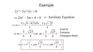
Case III: For complex roots ($m = \alpha \pm i\beta$), the solution encompasses oscillatory behavior:
$$ y = e^{\alpha x}(C_1 \cos(\beta x) + C_2 \sin(\beta x)) $$
Each case's solution reflects the nature of the roots derived from the auxiliary equation and serves foundationally in many engineering contexts. The examples provided emphasize the practical application of these solutions.
Youtube Videos


Audio Book
Dive deep into the subject with an immersive audiobook experience.
General Form of Homogeneous Equations
Chapter 1 of 4
🔒 Unlock Audio Chapter
Sign up and enroll to access the full audio experience
Chapter Content
The general form of a homogeneous equation with constant coefficients is given by:
d²y/dx² + b dy/dx + c y = 0.
Detailed Explanation
Homogeneous equations of this type involve the dependent variable y and its derivatives, where the coefficients (a, b, c) are constants. The equation shows how the changes in y are related to its second derivative (which measures acceleration) and first derivative (which measures velocity). This structure is important because it allows us to predict the behavior of various physical systems in engineering.
Examples & Analogies
Think of a simple mechanical system like a swing. The movement of the swing can be described by a similar second-order equation. Just like understanding how the swing moves back and forth can help create safer playgrounds, understanding this equation helps engineers design stable structures.
Auxiliary Equation (AE)
Chapter 2 of 4
🔒 Unlock Audio Chapter
Sign up and enroll to access the full audio experience
Chapter Content
To solve the homogeneous equation, we form the auxiliary equation (AE):
am² + bm + c = 0
and solve for roots m₁ and m₂.
Detailed Explanation
The auxiliary equation is a simplified polynomial form derived from the differential equation. By treating the equation as a standard quadratic equation, we can find the roots, which indicate the fundamental solutions of the original differential equation. The nature of these roots (real, equal, or complex) influences the form of the general solution.
Examples & Analogies
Imagine trying to find the roots of a quadratic equation like a treasure map. Each root you find leads you to a different solution point. If the roots are real and distinct, it's like finding two treasure spots; if they are complex, it indicates a hidden path in a mystical realm. Understanding the roots gives you guidance on the best way to approach the problem.
Cases Based on Roots of AE
Chapter 3 of 4
🔒 Unlock Audio Chapter
Sign up and enroll to access the full audio experience
Chapter Content
The roots of the auxiliary equation can lead to different general solution forms:
- Case I: Real and distinct roots (m₁, m₂) → y = C₁e^(m₁x) + C₂e^(m₂x)
- Case II: Real and equal roots (m) → y = (C₁ + C₂x)e^(mx)
- Case III: Complex roots (m = α ± iβ) → y = e^(αx)(C₁ cos(βx) + C₂ sin(βx))
Detailed Explanation
Each case corresponds to a different behavior of the solution based on the roots. In Case I, the distinct roots imply two independent solutions that combine to provide the complete response. In Case II, equal roots introduce an additional factor of x to account for the repeated nature of the root. In Case III, complex roots suggest oscillatory behavior in the solution, typical in systems that exhibit wave-like properties.
Examples & Analogies
Consider a violin string being plucked. The different cases represent different ways the string vibrates. In the first case, you hear a clear tone (distinct roots), in the second, you get a dulled, prolonged sound (equal roots), and in the third case, you hear a rich mixture of tones and harmonics (complex roots) – much like how different roots shape the behavior of physical systems.
Example of Solving Homogeneous Equation
Chapter 4 of 4
🔒 Unlock Audio Chapter
Sign up and enroll to access the full audio experience
Chapter Content
For the equation:
d²y/dx² - 5 dy/dx + 6y = 0,
the auxiliary equation is:
m² - 5m + 6 = 0 → m = 2, 3.
Thus, the general solution is:
y = C₁e^(2x) + C₂e^(3x).
Detailed Explanation
In this example, we first convert the homogeneous differential equation into its auxiliary form to find the roots. We then apply the identified roots to construct the general solution. Each constant (C₁, C₂) represents a certain degree of freedom in the system's response, indicating that there can be many possible solutions depending on initial conditions.
Examples & Analogies
Imagine tuning a guitar string. Depending on how tightly you pull the string (the constants C₁ and C₂ represent different tensions), the pitch will change. Just as a string can resonate at different frequencies, the solutions to our equation reflect how a physical system can behave in different scenarios.
Key Concepts
-
Homogeneous Equation: A differential equation set to zero, having no external forces.
-
Auxiliary Equation: A quadratic equation derived to find roots that inform the general solution.
-
Cases of Roots: The nature of roots (real, equal, complex) determines the structure of the general solution.
Examples & Applications
Example 1: Solve the equation d²y/dx² - 5 dy/dx + 6y = 0, leading to the general solution y = C₁ e^(2x) + C₂ e^(3x).
Example 2: The general solution derived from complex roots would look like y = e^(αx)(C₁ cos(βx) + C₂ sin(βx)).
Memory Aids
Interactive tools to help you remember key concepts
Rhymes
For real roots that are distinct and bold, Exponential solutions unfold.
Stories
Imagine a boat on still waters (homogeneous) affected only by wind (no external forces). When waters ripple (roots), the waves change (solution forms).
Memory Tools
To remember the types of roots: 'DR (Distinct Real)', 'ER (Equal Real)', and 'CR (Complex Roots)'.
Acronyms
H.E.A.R (Homogeneous Equations are Real) to recap the properties of homogeneous equations.
Flash Cards
Glossary
- Homogeneous Equation
A differential equation which has the form where all terms are proportional to the unknown function or its derivatives, set equal to zero.
- Auxiliary Equation (AE)
A quadratic equation derived from a linear differential equation used to find the roots which indicate the behavior of the solution.
- Roots
The values of 'm' found from the auxiliary equation that affect the form of the solution to the original differential equation.
- Real and Distinct Roots
Roots of the auxiliary equation that are different from each other and lead to exponential solutions.
- Complex Roots
Roots of the auxiliary equation that include imaginary parts, resulting in solutions that incorporate trigonometric functions.
Reference links
Supplementary resources to enhance your learning experience.