
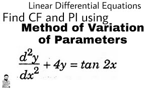
Method of Variation of Parameters
Enroll to start learning
You’ve not yet enrolled in this course. Please enroll for free to listen to audio lessons, classroom podcasts and take practice test.
Interactive Audio Lesson
Listen to a student-teacher conversation explaining the topic in a relatable way.
Introduction to the Method of Variation of Parameters
🔒 Unlock Audio Lesson
Sign up and enroll to listen to this audio lesson

Today, we're learning about the method of variation of parameters. This is a crucial technique for solving non-homogeneous linear differential equations, especially when simpler methods are unsuitable. Has anyone heard about this method before?

I think I've seen it mentioned in textbooks, but I'm not sure how it works.

What kind of problems does it solve?
Great questions! This method allows us to build particular solutions when the non-homogeneous term isn't a simple polynomial or exponential. Its flexibility makes it very practical in engineering applications.

Can you give us an example of when to use this method?
Absolutely! If we're given a term like sin(x), which doesn't fit into the method of undetermined coefficients, we can turn to variation of parameters.

How does this method differ from the others?
That's an important point to consider. While other methods often rely on guessing forms for particular solutions, variation of parameters systematically constructs those particular solutions using the complementary solution.
Setting Up the Problem
🔒 Unlock Audio Lesson
Sign up and enroll to listen to this audio lesson

Now that we have the introduction down, let’s look at how we set up the problem. If we have a complementary solution like $y_c = C_1y_1(x) + C_2y_2(x)$, we substitute it into our particular solution form. What do we replace the constants with?
We replace C_1 and C_2 with functions, right?
Exactly! So we formulate it as $y_p = u_1(x)y_1(x) + u_2(x)y_2(x)$. Next, we differentiate it. Does anyone recall what the next step is?
We have to set up equations using these functions?
That's correct! We set up the system of equations to solve for $u_1'$ and $u_2'$, which leads us to the formulae for our new functions.
What are those equations again?
"They are:
Solving the System of Equations
🔒 Unlock Audio Lesson
Sign up and enroll to listen to this audio lesson
Let’s dive into solving the equations. How can we isolate $u_1'$ and $u_2'$ from our system of equations?
We probably need to express one in terms of the other first?
Exactly right! By manipulating the first equation, we can express $u_2'$ in terms of $u_1'$ and substitute into the second equation. This forms a more solvable equation.
What happens after we find $u_1$ and $u_2$?
Great question! After determining those functions, we substitute them back into our expression for the particular solution $y_p$.
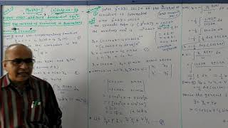
Example Problem
🔒 Unlock Audio Lesson
Sign up and enroll to listen to this audio lesson
Now, let's solve an example using variation of parameters. Consider the equation $y'' + 2y' + y = e^x$. What are our first steps?
We need to find the complementary solution first.
Yes! Then we find $y_c$ and identify $R(x) = e^x$.
After that, we can set up our expressions for $u_1$ and $u_2$.
Exactly! By following the steps we discussed, we can find $y_p$, and then we can combine it with $y_c$ to find the general solution.
Recap and Key Insights
🔒 Unlock Audio Lesson
Sign up and enroll to listen to this audio lesson
To conclude, can anyone summarize the steps of the method of variation of parameters?
We first find the complementary solution, then express our particular solution with functions, set up equations, solve for those functions, and finally substitute back!
It seems like a powerful method for more complex differential equations!
Absolutely! This method ensures we can tackle a wide range of non-homogeneous problems. Remember, practice is key to mastery!
Introduction & Overview
Read summaries of the section's main ideas at different levels of detail.
Quick Overview
Standard
This section discusses the method of variation of parameters for solving non-homogeneous linear differential equations. It explains how to derive a particular solution based on the complementary solution and the non-homogeneous term, laying out the steps needed to determine new functions that act as coefficients for this solution.
Detailed
Method of Variation of Parameters
The method of variation of parameters is employed when finding particular solutions to non-homogeneous linear differential equations, particularly when the non-homogeneous term isn't suitable for the method of undetermined coefficients. In this method, if the complementary solution for the corresponding homogeneous equation is given by:
$$y_c = C_1y_1(x) + C_2y_2(x)$$
The particular solution is constructed in the form:
$$y_p = u_1(x)y_1(x) + u_2(x)y_2(x)$$
where $u_1(x)$ and $u_2(x)$ are functions to be determined from the differential equation. The system of equations to solve for these functions is:
- $$u_1'y_1 + u_2'y_2 = 0$$
- $$u_1'y_1' + u_2'y_2' = R(x)$$
This method allows flexibility in handling non-homogeneous terms that do not conform to simple polynomial, exponential, or trigonometric forms, providing engineers with a robust tool for modeling complex systems.
Youtube Videos


Audio Book
Dive deep into the subject with an immersive audiobook experience.
Overview of the Method
Chapter 1 of 3
🔒 Unlock Audio Chapter
Sign up and enroll to access the full audio experience
Chapter Content
Use when R(x) is not suitable for undetermined coefficients. If the homogeneous solution is:
y =C₁y₁(x)+C₂y₂(x)
Detailed Explanation
The Method of Variation of Parameters is a solution technique applied to non-homogeneous differential equations when the right-hand side (R(x)) is not suitable for the Method of Undetermined Coefficients. The primary goal here is to find a particular solution (yₕ) to complement the homogeneous solution. If the homogeneous solution has two parts, C₁y₁(x) and C₂y₂(x), where C₁ and C₂ are constants, we can adapt these constants into functions that vary with x, instead of being fixed constants.
Examples & Analogies
Imagine you are trying to balance a seesaw (the differential equation) that has weights (the function R(x)) positioned in various places. Sometimes, using fixed weights (undetermined coefficients) doesn't work effectively. Instead, you could use adjustable weights (varying parameters) that can slide along the seesaw, allowing for a balance despite the changing loads.
Form of the Particular Solution
Chapter 2 of 3
🔒 Unlock Audio Chapter
Sign up and enroll to access the full audio experience
Chapter Content
Then particular solution is:
yₚ=u₁(x)y₁(x)+u₂(x)y₂(x)
Detailed Explanation
Once we acknowledge the homogeneous solution, we seek a particular solution in the form of yₚ, which is constructed using the functions u₁(x) and u₂(x). These functions multiply the homogeneous solutions y₁(x) and y₂(x). The idea is that by allowing u₁ and u₂ to vary, we can better absorb the non-homogeneous term R(x) into the overall solution.
Examples & Analogies
Think of creating a custom sandwich. The bread (y₁(x)) and fillings (y₂(x)) are the base that everyone can use. However, you can choose unique toppings (u₁ and u₂) based on your preferences at different times, which allows you to cater to different tastes (the varying conditions of the differential equation) while still starting with the same basic sandwich.
Finding the Functions u₁ and u₂
Chapter 3 of 3
🔒 Unlock Audio Chapter
Sign up and enroll to access the full audio experience
Chapter Content
Where u₁, u₂ are found by solving:
{ u₁′y₁ + u₂′y₂ = 0
u₁′y₁ + u₂′y₂ = R(x) }
Detailed Explanation
To find the functions u₁ and u₂, we set up a system of equations based on the product rule of differentiation. The first equation ensures that the weighted combination of y₁ and y₂ does not change the structure of the homogeneous part, while the second equation captures the influence of the non-homogeneous term R(x). By solving this system, we can derive the expressions for u₁ and u₂ that allow the particular solution to effectively counterbalance the non-homogeneous part of the equation.
Examples & Analogies
Imagine you’re inventing a new recipe for a cake (the differential equation) but you want to keep the classic cake base (the homogeneous solution) intact. To adjust for flavor (R(x)), you create new topping options (u₁ and u₂) while ensuring the cake itself remains the same. The equations you set up are like writing a perfect shopping list that ensures you can adjust the flavor without losing the essence of the original cake.
Key Concepts
-
Variation of Parameters: A method for solving non-homogeneous equations.
-
Complementary Solution: The solution to the homogeneous part of the differential equation.
-
Particular Solution: Constructed solution based on variation of parameters.
-
System of Equations: Derived equations used to solve for new function coefficients.
Examples & Applications
Consider the equation y'' + y = sin(x). Using variation of parameters, we find the complementary solution first and then derive the particular solution using u_1 and u_2.
For the equation y'' - 3y' + 2y = e^x, we start with the complementary solution, then apply variation of parameters to derive a suitable y_p.
Memory Aids
Interactive tools to help you remember key concepts
Rhymes
When parameters vary, solutions are found, in the world of functions, where equations abound.
Stories
Imagine two friends, U1 and U2, who set out to solve the mystery of a tricky equation. They combined their knowledge, shaped it into a unique solution, and together conquered the challenge by varying their parameters!
Memory Tools
Use the mnemonic 'VAV' for 'Variation - Apply - Validate' to remember the steps in variation of parameters.
Acronyms
CUP for Complementary, Unrelated Functions, Parameters – to remember the critical aspects of solving using variation of parameters.
Flash Cards
Glossary
- Variation of Parameters
A method to find particular solutions to non-homogeneous linear differential equations when standard methods are not suitable.
- Complementary Solution
The solution to the corresponding homogeneous differential equation.
- NonHomogeneous Term
The part of a differential equation that does not involve the unknown function and its derivatives.
- Parameter
A variable that helps define specific conditions in a given context, often referring to the functions $u_1$ and $u_2$ in variation of parameters.
Reference links
Supplementary resources to enhance your learning experience.