
Second-Order Linear Differential Equations
Enroll to start learning
You’ve not yet enrolled in this course. Please enroll for free to listen to audio lessons, classroom podcasts and take practice test.
Interactive Audio Lesson
Listen to a student-teacher conversation explaining the topic in a relatable way.
General Form of Second-Order Linear Differential Equations
🔒 Unlock Audio Lesson
Sign up and enroll to listen to this audio lesson

Today we’re going to discuss the general form of second-order linear differential equations. Can anyone tell me what the general form looks like?

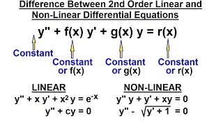
Isn’t it something like d²y/dx² + P(x) dy/dx + Q(x)y = R(x)?
Exactly! And this can be classified as either homogeneous or non-homogeneous depending on whether R(x) equals zero or not.

So what happens if R(x) is zero?
Great question! That means we are dealing with a homogeneous equation, which we'll solve differently. Remember: Homogeneous is like a house with no guests, but non-homogeneous has guests over, which is R(x)!

I like that analogy!
Let’s summarize: The general form is crucial for identifying how to approach the solution. Next, we will explore methods to find solutions, so stay tuned!
Homogeneous Equations and the Auxiliary Equation
🔒 Unlock Audio Lesson
Sign up and enroll to listen to this audio lesson

Now let’s dive deeper into homogeneous equations, specifically those with constant coefficients. What's the general form in this case?

It’s a²y″ + b y′ + cy = 0, right?
Correct! This leads to the Auxiliary Equation: am² + bm + c = 0. What do we do with this equation?
We solve for m to find roots, right?
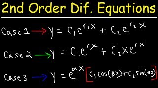
Exactly! Knowing the types of roots guides you to write your general solution. If we have distinct real roots, what’s the form?
It’s y = C₁e^(m₁x) + C₂e^(m₂x)!
Well done! Let’s recap: For distinct roots, we use an exponential form, which is an essential skill in engineering applications.
Non-Homogeneous Equations
🔒 Unlock Audio Lesson
Sign up and enroll to listen to this audio lesson
We’ve talked about homogeneous equations. Now, how do we approach a non-homogeneous equation?
We find a complementary function and then a particular solution, right?
Exactly! And the complete solution is y = yc + yp. What’s the complementary function derived from?
It comes from the homogeneous equation!
Spot on! And then we find yp. We often use undetermined coefficients or variation of parameters for that, but remember, the nature of R(x) helps us decide which method to use.
This is helpful for real applications, like structural analysis!
Absolutely! Each step we take reinforces our understanding of the behavior of systems in engineering.
Introduction & Overview
Read summaries of the section's main ideas at different levels of detail.
Quick Overview
Standard
The discussion on second-order linear differential equations covers their general forms, potential classifications as homogeneous or non-homogeneous, and effective solution methods including finding complementary functions and specific solutions. Practical applications are highlighted in the context of engineering.
Detailed
Detailed Summary
Second-order linear differential equations are equations of the form:
$$\frac{d^2y}{dx^2} + P(x) \frac{dy}{dx} + Q(x)y = R(x)$$
These equations play a critical role in modeling dynamic systems in civil engineering, such as vibrations in beams and deflection behaviors.
1.4.1 General Form
Each second-order differential equation can be classified as either homogeneous (where R(x) = 0) or non-homogeneous (where R(x) ≠ 0). This classification informs the solution approach.
1.5 Homogeneous Equations with Constant Coefficients
The homogeneous version has the standard form:
$$a\frac{d^2y}{dx^2} + b\frac{dy}{dx} + cy = 0$$
1.5.2 Auxiliary Equation (AE)
The associated auxiliary equation, defined as:
$$am^2 + bm + c = 0,$$
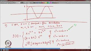
can possess different types of roots, leading to specific forms for the general solution, including distinct real roots, repeated roots, or complex roots.
1.5.3 Example
For instance, solving:
$$\frac{d^2y}{dx^2} - 5\frac{dy}{dx} + 6y = 0$$
involves using the auxiliary equation to find the roots and subsequently formulating the general solution based on those roots.
1.6 Non-Homogeneous Linear Equations
Non-homogeneous equations require the overall solution to consist of a complementary function (from the homogeneous part) plus a particular solution determined through various methods.
1.7 Methods of Finding Particular Solutions
Methods such as the undetermined coefficients and variation of parameters provide systematic ways to derive particular solutions based on the nature of R(x).
Engineering Applications
These equations are pivotal in applications such as beam deflection, fluid dynamics, and structural vibrations.
Youtube Videos


![Ordinary Differential Equations 25 | Example for Non-Diagonalizable Matrix [dark version]](https://img.youtube.com/vi/aPcCF1a21IU/mqdefault.jpg)
Audio Book
Dive deep into the subject with an immersive audiobook experience.
General Form of Second-Order Linear Differential Equations
Chapter 1 of 2
🔒 Unlock Audio Chapter
Sign up and enroll to access the full audio experience
Chapter Content
The general form of a second-order linear differential equation is:
$$\frac{d^2y}{dx^2} + P(x) \frac{dy}{dx} + Q(x)y = R(x)$$
This can be homogeneous (when $R(x) = 0$) or non-homogeneous.
Detailed Explanation
The general form of a second-order linear differential equation captures the relationship between a function and its derivatives. Specifically, the equation includes the second derivative of a function, the first derivative, the function itself, and an external influence (denoted as R(x)). A key point is whether R(x) is zero or non-zero; if it is zero, the equation is considered homogeneous, indicating that the solutions depend solely on the function and its derivatives. If R(x) is non-zero, the equation is non-homogeneous, meaning there is an external factor influencing the system.
Examples & Analogies
Consider a simple spring-mass system in physics. If you attach a spring to a weight hanging from a ceiling, the motion of the weight can be described by a second-order linear differential equation. In the case of just the spring's force acting on the weight (no additional forces), the equation is homogeneous. However, if an external force, like a pushing hand, is introduced, it becomes non-homogeneous.
Homogeneous vs Non-Homogeneous
Chapter 2 of 2
🔒 Unlock Audio Chapter
Sign up and enroll to access the full audio experience
Chapter Content
In a homogeneous equation, $R(x) = 0$, meaning that the equation simplifies to:
$$\frac{d^2y}{dx^2} + P(x) \frac{dy}{dx} + Q(x)y = 0$$
In contrast, a non-homogeneous equation includes a non-zero function $R(x)$.
Detailed Explanation
Homogeneous second-order linear differential equations showcase systems that return to equilibrium when disturbed. The absence of external influences described by R(x) means that solutions are solely derived from initial conditions or inherent properties of the system. On the other hand, non-homogeneous equations consider external influences or forces acting on the system, thus requiring solutions that incorporate these factors to accurately predict behavior over time.
Examples & Analogies
Imagine a swing. When you push it (like R(x) being non-zero), it moves due to your force. If you stop pushing (R(x) equals zero), the swing's motion relies purely on its initial position and the force of gravity, representing a homogeneous situation.
Key Concepts
-
Second-Order Linear Differential Equations: These equations define relationships involving a function and its derivatives up to the second degree and can be structured to reflect various conditions based on their coefficients.
-
Homogeneous vs Non-Homogeneous: Understanding the difference between these two forms of equations is critical to correctly applying solution techniques.
-
Auxiliary Equation: The formation of an auxiliary equation from a homogeneous differential equation is crucial to finding roots which lead to general solutions.
Examples & Applications
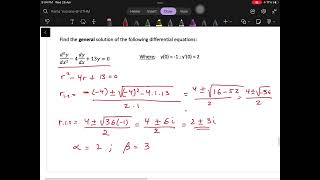
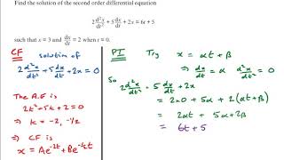
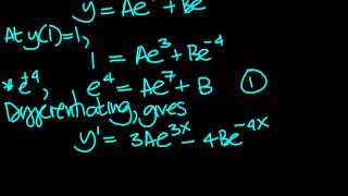
Example 1: Solve the homogeneous equation d²y/dx² - 5 dy/dx + 6y = 0. The auxiliary equation is m² - 5m + 6 = 0, yielding the roots m = 2 and m = 3. The general solution is y = C₁e²x + C₂e³x.
Example 2: For a non-homogeneous equation d²y/dx² - 5 dy/dx + 6y = e^x, first find the complementary function as detailed in Example 1, then apply a method such as undetermined coefficients for yp.
Memory Aids
Interactive tools to help you remember key concepts
Rhymes
A second-order need, it's plain to see, where roots are defined, solutions flow free.
Stories
Imagine a gear turning, it's the same every time (homogeneous) unless you add a hand to push (non-homogeneous), defining new paths to climb.
Memory Tools
To remember types of roots: 'Real, Repeat, or Complex', just think of a river that bends, merges, or wraps!
Acronyms
R.E.C. for Roots
Real
Equal
Complex helps recall the forms we seek.
Flash Cards
Glossary
- SecondOrder Linear Differential Equation
An equation involving a dependent variable y and its derivatives up to the second order, which can be written in the form d²y/dx² + P(x)dy/dx + Q(x)y = R(x).
- Homogeneous Equation
A differential equation where R(x) = 0, indicating that all terms are dependent on the function y and its derivatives.
- NonHomogeneous Equation
A differential equation where R(x) ≠ 0, indicating the presence of an external input or forcing function.
- Auxiliary Equation
An algebraic equation derived from a homogeneous linear differential equation, used to find the roots that help form the general solution.
- Complementary Function
The solution to the corresponding homogeneous equation, which is part of the general solution for non-homogeneous equations.
- Particular Solution
A specific solution to the non-homogeneous equation that satisfies the original differential equation.
Reference links
Supplementary resources to enhance your learning experience.