
First-Order Linear Differential Equations
Enroll to start learning
You’ve not yet enrolled in this course. Please enroll for free to listen to audio lessons, classroom podcasts and take practice test.
Interactive Audio Lesson
Listen to a student-teacher conversation explaining the topic in a relatable way.
Understanding the General Form
🔒 Unlock Audio Lesson
Sign up and enroll to listen to this audio lesson

Welcome everyone! Today, we will focus on first-order linear differential equations. They typically look like this: dy/dx + P(x)y = Q(x). Can anyone tell me what P(x) and Q(x) represent?

P(x) is the coefficient of y, and Q(x) is a function that describes the external influence on the system, right?
Exactly! P(x) affects how y changes, while Q(x) represents external forces or inputs. Remember this format as it is key to solving these equations.

So if I see this form, I know it’s a first-order linear differential equation?
That’s correct! Now, let’s move on to the integrating factor method used to solve these equations.
Using the Integrating Factor Method
🔒 Unlock Audio Lesson
Sign up and enroll to listen to this audio lesson

To solve a first-order linear differential equation, we use the integrating factor, µ(x). This is calculated as µ(x) = e^(∫P(x)dx). Any thoughts on why this is necessary?

I think it transforms the equation into a more workable form?
Absolutely! By multiplying both sides by µ(x), we simplify our equation to something we can integrate easily. Let’s practice this with our previous equation.

How do we actually perform the integration after applying the factor?
Great question! After multiplying, we integrate both sides. This gives us the solution y. Let’s go through the example together.
Step-by-Step Example
🔒 Unlock Audio Lesson
Sign up and enroll to listen to this audio lesson
Let’s take our example: dy/dx + 2y = e^(-x). First, we identify P(x) and calculate the integrating factor. What’s P(x) here?
P(x) is 2.
Correct! Now, calculating µ(x): e^(∫2dx) = e^(2x). Now, what do we do next?
We multiply both sides by e^(2x).
Exactly! That rewrites our equation as d[e^(2x)*y]/dx = e^(x). Let’s integrate both sides now.
General Solution and Conclusion
🔒 Unlock Audio Lesson
Sign up and enroll to listen to this audio lesson
After integration, we found e^(2x)*y = e^(x) + C. How would you isolate y?
By dividing both sides by e^(2x).
Correct! This results in y = e^(-x) + Ce^(-2x), which is our general solution. Can anyone summarize why the integrating factor is so useful?
It allows us to transform the equation into a form we can easily integrate.
Exactly! This method is vital in finding solutions to first-order linear differential equations. Remember this process!
Introduction & Overview
Read summaries of the section's main ideas at different levels of detail.
Quick Overview
Standard
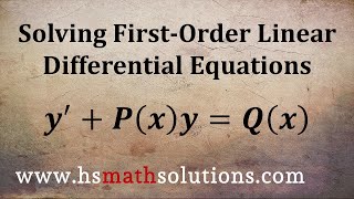
First-order linear differential equations, expressed in the form dy/dx + P(x)y = Q(x), are explored in this section along with the integrating factor method, step-by-step solutions, and an illustrative example demonstrating the process.
Detailed
Overview of First-Order Linear Differential Equations
First-order linear differential equations are fundamental in various applications within civil engineering. They are expressed in the format:
General Form:
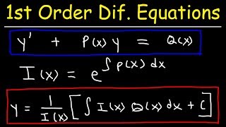
dy/dx + P(x)y = Q(x)
This equation involves a dependent variable y, an independent variable x, and functions P(x) and Q(x) that are defined in the context of the problem.
Solution Method: The Integrating Factor
The traditional approach to solve first-order linear differential equations relies on the acquiring of an integrating factor (IF), denoted as µ(x). The step-by-step method involves:
- Calculate the Integrating Factor:
- µ(x) = e^(∫P(x)dx)
- Reformulate the Equation:
-
This transforms the equation into the format:
d[µ(x)y]/dx = µ(x)Q(x)
- Integrate:
-
∫d[µ(x)y] = ∫µ(x)Q(x)dx
- This provides the general solution for y.
Example Solved
For example, for the equation:
dy/dx + 2y = e^(-x),
we follow the steps to arrive at the solution y = e^(-x) + Ce^(-2x).
This section provides a solid foundation for understanding how first-order linear differential equations function and their resolution in practical scenarios.
Youtube Videos


![Ordinary Differential Equations 25 | Example for Non-Diagonalizable Matrix [dark version]](https://img.youtube.com/vi/aPcCF1a21IU/mqdefault.jpg)


Audio Book
Dive deep into the subject with an immersive audiobook experience.
General Form
Chapter 1 of 3
🔒 Unlock Audio Chapter
Sign up and enroll to access the full audio experience
Chapter Content
The general form of a first-order linear differential equation is:
$$\frac{dy}{dx} + P(x)y = Q(x)$$
Detailed Explanation
In this equation, \( y \) is the unknown function that depends on \( x \), and it can be thought of as a dependent variable. The function \( P(x) \) is a given function that multiplies with \( y \), and \( Q(x) \) is another given function that can be seen as a source term. This equation essentially describes how the rate of change of the variable \( y \) relates to its current state and the influences represented by \( P(x) \) and \( Q(x) \).
Examples & Analogies
Imagine a tank that is being filled with water. The amount of water in the tank at any time \( y \) is influenced by both the speed at which water flows in (represented by \( Q(x) \)) and the existing pressure or flow conditions inside the tank (represented by \( P(x) \)).
Solution Method: Integrating Factor (IF)
Chapter 2 of 3
🔒 Unlock Audio Chapter
Sign up and enroll to access the full audio experience
Chapter Content
To solve the equation, the standard method involves the following steps:
- Multiply both sides by an integrating factor:
$$\mu(x) = e^{\int P(x)dx}$$ - This transforms the equation into:
$$\frac{d}{dx}[\mu(x)y] = \mu(x)Q(x)$$ - Integrate both sides:
$$y = \frac{1}{\mu(x)}\int \mu(x)Q(x)dx + C$$
Detailed Explanation
The integrating factor \( \mu(x) \) is calculated based on the function \( P(x) \). This integrating factor serves to simplify the left side of the equation so that it can be expressed as the derivative of a product. After multiplying by \( \mu(x) \), the equation can be integrated, yielding a solution for \( y \) in terms of an integral involving \( Q(x) \) and the integrating factor itself, along with an arbitrary constant \( C \). This constant represents the general solution's family of curves.
Examples & Analogies
If we think of a car's speedometer, the rate of change of speed can depend on various factors such as acceleration and road conditions. By determining an integrating factor (like using additional information such as fuel consumption rates), we can better predict the car's speed over time, leading to a clearer understanding of its behavior under different conditions.
Example of Solving a First-Order Linear DE
Chapter 3 of 3
🔒 Unlock Audio Chapter
Sign up and enroll to access the full audio experience
Chapter Content
Consider the differential equation:
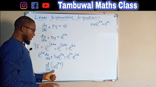
$$\frac{dy}{dx} + 2y = e^{-x}$$
Solution:
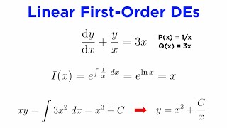
1. Identify \( P(x) = 2 \), thus \( \mu(x) = e^{\int 2dx} = e^{2x} \).
2. Multiply both sides:
$$e^{2x}\frac{dy}{dx} + 2e^{2x}y = e^{x}$$
3. Rewrite as:
$$\frac{d}{dx}(e^{2x}y) = e^{x}$$
4. Integrate both sides:
$$e^{2x}y = \int e^{x}dx + C$$
5. Solve:
$$y = e^{-x} + Ce^{-2x}$$
Detailed Explanation
In this example, we begin by determining the appropriate integrating factor based on the function \( P(x) = 2 \). Once we have calculated \( \mu(x) \), we multiply the entire differential equation by it, transforming our equation to expose the derivative on the left. After this transformation, we integrate both sides to find the general solution for \( y \) with an arbitrary constant.
Examples & Analogies
If we think about cooling a cup of coffee, the rate at which the coffee cools down is affected by the current temperature (which can be analogous to \( y \)). The outside environment (like air temperature) plays a role too (analogous to \( Q(x) \)). Using the integrating factor can be thought of as recognizing how these external influences change the cooling rate over time, helping us reach a clearer conclusion about the coffee's temperature changes.
Key Concepts
-
General Form of First-Order DE: dy/dx + P(x)y = Q(x) is key to identifying the type of differential equation.
-
Integrating Factor: µ(x) allows us to manipulate the equation for easier integration.
-
Solution Process: Step-by-step integration leads to the general solution.
Examples & Applications
Example 1: Solve dy/dx + 2y = e^(-x). Solution yields y = e^(-x) + Ce^(-2x).
Memory Aids
Interactive tools to help you remember key concepts
Rhymes
When solving DE as first-rate, find P, then integrate!
Stories
Imagine a sailor, lost at sea; he finds his path by the wind’s decree. P leads the way, guiding his ship, while Q gives the currents a proper grip!
Memory Tools
To remember the integrating factor: Calculate, Multiply, Integrate!
Acronyms
M.I.S. - Multiply, Integrate, Solve for differential equations.
Flash Cards
Glossary
- Differential Equation
An equation involving an unknown function and its derivatives.
- FirstOrder Linear DE
A type of differential equation where the highest derivative is the first order and is linear in nature.
- Integrating Factor
A function used to multiply a differential equation to facilitate integration.
- General Solution
The most general form of the solution of a differential equation, containing constants.
Reference links
Supplementary resources to enhance your learning experience.