
General Procedure
Enroll to start learning
You’ve not yet enrolled in this course. Please enroll for free to listen to audio lessons, classroom podcasts and take practice test.
Interactive Audio Lesson
Listen to a student-teacher conversation explaining the topic in a relatable way.
Assuming a Solution
🔒 Unlock Audio Lesson
Sign up and enroll to listen to this audio lesson

Today, we'll explore how to use the separation of variables technique effectively. The first step is to assume a solution for our PDE. Can anyone tell me how we might express this assumption?

We can assume a solution of the form \( u(x, t) = X(x) T(t) \) right?
Exactly, well done! This representation allows us to break our problem into more manageable parts based on different variables. Now, why do we think this is a good assumption?

Because it simplifies the equation into two functions, making it easier to solve?
Precisely! When we assume a product form, we can explore the behavior of each variable independently. Remember, we'll substitute this into our PDE next.
Substituting into the PDE
🔒 Unlock Audio Lesson
Sign up and enroll to listen to this audio lesson

Moving on, after assuming our solution, what comes next?

We need to substitute \( u(x, t) = X(x) T(t) \) into the PDE!
Correct! By substituting, we set the stage to separate our variables. This manipulation is crucial. What do we aim to achieve after this step?

We want to rearrange it into parts that depend only on \( x \) or \( t \).
Exactly! Once we've separated the variables, it leads us to distinct ordinary differential equations that we can solve.
Solving the ODEs
🔒 Unlock Audio Lesson
Sign up and enroll to listen to this audio lesson
Now that we have our separated equations, how do we move forward?
We can solve each ordinary differential equation separately.
That's right! We typically end up with one ODE in terms of \( x \) and another in terms of \( t \). Can anyone think about why solving them individually is advantageous?
It allows us to focus on one variable at a time without the complexity of the other.
Exactly! This strategy simplifies the analysis. Let's think about boundary conditions next, which are vital for our solution.
Applying Boundary Conditions
🔒 Unlock Audio Lesson
Sign up and enroll to listen to this audio lesson
Now we come to a critical part: applying boundary conditions. Why is this a necessary step?
To find the specific values for \( \lambda \) and to ensure the solutions fit the physical problems we're dealing with.
Very good! Boundary conditions help specify the form of the solution and make it unique. How do we apply these conditions?
We substitute our solutions back into the boundary equations to see what restrictions we have.
Exactly! This will lead us to specific eigenfunctions and their corresponding eigenvalues.
Constructing the General Solution
🔒 Unlock Audio Lesson
Sign up and enroll to listen to this audio lesson
Finally, after we have our eigenfunctions, what do we do to wrap everything up?
We construct the general solution as a series using superposition.
Correct! This principle allows us to add multiple solutions together, leading us back to our original variables. Why is this step beneficial?
It enables us to represent more complex behaviors through simpler components.
Exactly! And remember, we’ll often use Fourier series to express these complex functions. Great work today, everyone!
Introduction & Overview
Read summaries of the section's main ideas at different levels of detail.
Quick Overview
Standard
The general procedure for applying the method of separation of variables involves assuming solutions in the form of products of single-variable functions, substituting them into the PDE, solving the resulting ordinary differential equations (ODEs), and applying boundary conditions to construct a general solution. This systematic approach allows engineers to tackle complex civil engineering problems.
Detailed
General Procedure for Separation of Variables
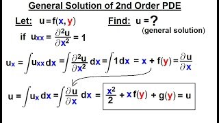
- Assume a Solution: We start by hypothesizing that the solution of a given PDE can be expressed as a product of two functions - one dependent on one variable (e.g., space) and another dependent on another variable (e.g., time). This is denoted as
\[ u(x, t) = X(x)T(t) \]
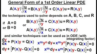
- Substitute into the PDE: We then substitute this product back into the given partial differential equation. This step transforms the equation into a form where separation is possible.
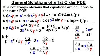
- Separate the Variables: Next, we manipulate the equation to arrange it in a way that each side depends solely on one variable, resulting in a form that includes a separation constant \( \lambda \). This step typically leads to two separate ordinary differential equations (ODEs).
- Solve the ODEs: After separation, each of the resulting ODEs can be solved individually, providing the respective solutions for \( X(x) \) and \( T(t) \).
- Apply Boundary Conditions: The solutions obtained must be verified against given boundary conditions to determine specific values for the separation constant \( \lambda \) and corresponding eigenfunctions that satisfy these conditions.
- Construct the General Solution: Finally, the general solution is constructed by summing the individual solutions (using the principle of superposition), which leads to a complete expression for the original problem. This method, particularly when combined with Fourier series, provides a powerful tool for engineers to model and analyze complex phenomena in civil engineering.
Youtube Videos


Audio Book
Dive deep into the subject with an immersive audiobook experience.
Assumption of Solution Form
Chapter 1 of 6
🔒 Unlock Audio Chapter
Sign up and enroll to access the full audio experience
Chapter Content
- Assume a solution of the form:
u(x,t)=X(x)T(t)
Detailed Explanation
In the method of separation of variables, the first step is to assume that the solution to the partial differential equation (PDE) can be expressed as a product of two functions. The function u(x,t) represents the solution that depends on two variables: x and t. By setting u(x,t) as the product of X(x), which depends only on x, and T(t), which depends only on t, we simplify our task of solving the PDE. This approach allows us to tackle the problem in a more manageable way, focusing on one variable at a time.
Examples & Analogies
Imagine you're trying to solve a puzzle that’s too complicated to just look at once. Instead, you break it down into smaller sections. By focusing on one piece at a time (like focusing on X(x) and T(t)), it becomes easier to manage and eventually solve the entire puzzle.
Substitution into the PDE
Chapter 2 of 6
🔒 Unlock Audio Chapter
Sign up and enroll to access the full audio experience
Chapter Content
- Substitute into the PDE.
Detailed Explanation
After assuming the solution has the form u(x,t) = X(x)T(t), the next step is to substitute this form into the original PDE. This means replacing u in the PDE with X(x)T(t) and deriving the new equation resulting from this substitution. This new equation will typically involve partial derivatives of T(t) with respect to time and X(x) with respect to space. The goal here is to create an equation where each side can be separated into functions of a single variable.
Examples & Analogies
Think of substituting values into a recipe. If a recipe calls for 'x' cups of flour, and you've decided to break down the recipe into parts, you would replace 'x' in the recipe with the specific amount you need in that particular step. This makes the process clearer and allows you to focus on individual ingredients, just like we are focusing on the variables in our PDE.
Separation of Variables
Chapter 3 of 6
🔒 Unlock Audio Chapter
Sign up and enroll to access the full audio experience
Chapter Content
- Separate the equation such that each side depends on only one variable:
1 dT 1 d2X
= =−λ
T(t) dt X(x) dx2
• where λ is the separation constant.
Detailed Explanation
In this step, we rearrange the substituted PDE to isolate terms that only involve T(t) on one side and those that only involve X(x) on the other side. This is critical because it leads to two ordinary differential equations (ODEs). The introduction of the separation constant λ allows us to state that the relationship between the two variables is proportional, enabling us to solve them independently. This separation is key to simplifying the problem and making it more tractable.
Examples & Analogies
Consider a seesaw balanced in the middle. The left side only contains the weight of the left child (representing X(x)), and the right side only contains the weight of the right child (representing T(t)). By adjusting the weights on either side, you can analyze how each child affects the seesaw independently, just like how we separate variables to understand their individual contributions.
Solving the Resulting ODEs
Chapter 4 of 6
🔒 Unlock Audio Chapter
Sign up and enroll to access the full audio experience
Chapter Content
- Solve the resulting ODEs:
• One in x
• One in t
Detailed Explanation
Once we have successfully separated the PDE into two distinct equations—one involving only the spatial variable x and the other involving the temporal variable t—we can now solve these ordinary differential equations (ODEs) independently. This involves applying standard techniques for solving ODEs, which may include methods like integrating factors, characteristic equations, or even known solutions for specific types of equations. This step is crucial, as it provides us with functions that describe the behavior of our system over time and space.
Examples & Analogies
Think of a music piece that is divided into sections for different instruments. Each instrument plays its part independently, allowing musicians to focus on their specific sections before bringing the entire composition together. Similarly, we solve each ODE separately to understand different aspects of the original problem.
Applying Boundary Conditions
Chapter 5 of 6
🔒 Unlock Audio Chapter
Sign up and enroll to access the full audio experience
Chapter Content
- Apply boundary conditions to determine allowed values of λ and corresponding eigenfunctions.
Detailed Explanation
After finding the solutions to our ODEs, we now need to apply the boundary conditions relevant to our original problem to find specific values for the separation constant λ and the eigenfunctions associated with these values. These boundary conditions are essential because they ensure that the solution meets the physical realities of the problem—like temperatures being set at certain values at specific points or the behavior of a system at its edges. This step often yields a discrete set of allowed values for λ, which corresponds to unique solutions that fit the original PDE.
Examples & Analogies
Imagine a gardener who has specific plots of land defined by fences (the boundary conditions) that dictate where flowers can grow. Each flower type may only thrive in certain segments of the garden. Similarly, applying boundary conditions helps us discover where our mathematical solutions can 'grow' and fit into the larger context of our problem.
Constructing the General Solution
Chapter 6 of 6
🔒 Unlock Audio Chapter
Sign up and enroll to access the full audio experience
Chapter Content
- Construct the general solution as a series using the principle of superposition.
Detailed Explanation
The final step in the separation of variables procedure is to construct the general solution to the original PDE using the solutions derived from the ODEs and the identified eigenfunctions. This is done through a process known as superposition, where we add together these individual solutions, each scaled by corresponding coefficients based on the initial conditions. This combined solution represents the overall behavior of the system over the defined domain and satisfies all imposed boundary and initial conditions.
Examples & Analogies
Think of creating a smoothie by blending different fruits together. Each fruit adds its unique flavor and contributes to the overall taste of the smoothie. By combining them, you create a delicious mix that is greater than the sum of its parts, much like how we use the principle of superposition to combine various solutions into one comprehensive answer.
Key Concepts
-
Separation of Variables: A method to solve PDEs by assuming solutions as products of single-variable functions.
-
Boundary Conditions: Constraints applied at the edges of a domain that must be satisfied by the solution.
-
Eigenfunctions: Functions derived from the separated equations that give insight into the behavior of the system.
Examples & Applications
When solving the heat equation, we often assume a solution of the form u(x,t) = X(x)T(t) to separate space and time variables.
Considering boundary conditions like u(0,t) = 0 can help determine specific values of λ in the solution.
Memory Aids
Interactive tools to help you remember key concepts
Rhymes
To solve a PDE with ease, assume a product, if you please.
Stories
Imagine a wise engineer sailing a river; first, she splits her route into two paths - one for water, one for wind – before docking at the shore, she checks the conditions at the banks.
Memory Tools
Remember 'ASSETS' for the general procedure: Assume, Substitute, Separate, Solve, Apply, THE (Boundary Conditions), and Sum.
Acronyms
P.A.S.S. - Assume, Substitute, Separate, Solve.
Flash Cards
Glossary
- Partial Differential Equation (PDE)
An equation that involves partial derivatives of a multivariable function.
- Ordinary Differential Equation (ODE)
A differential equation containing one independent variable.
- Eigenfunction
A non-zero function that changes at most by a scalar factor when an operator is applied to it.
- Boundary Condition
A constraint necessary to solve a PDE, applied at the boundaries of the domain.
- Separation Constant (λ)
A constant introduced during the process of variable separation, helping in formulating separated equations.
Reference links
Supplementary resources to enhance your learning experience.