
Separation of Variables, Use of Fourier Series
Enroll to start learning
You’ve not yet enrolled in this course. Please enroll for free to listen to audio lessons, classroom podcasts and take practice test.
Interactive Audio Lesson
Listen to a student-teacher conversation explaining the topic in a relatable way.
Introduction to Partial Differential Equations
🔒 Unlock Audio Lesson
Sign up and enroll to listen to this audio lesson

Welcome to our session! Today, we're diving into Partial Differential Equations or PDEs. Can anyone tell me what a PDE is?

Is it an equation that involves partial derivatives of a function of multiple variables?
Correct! PDEs govern many physical phenomena. They can be classified as elliptic, parabolic, or hyperbolic. What are some examples you remember related to civil engineering?

Laplace's equation for steady-state heat distribution is an elliptic PDE.

And the wave equation for vibrations is a hyperbolic PDE.
Great! These classifications help determine the appropriate solution methods. Remember: Elliptic = steady-state, Parabolic = time-dependent, Hyperbolic = waves.
Let's recap: PDEs involve multiple variables and can be classified based on their types. Any questions?
Method of Separation of Variables
🔒 Unlock Audio Lesson
Sign up and enroll to listen to this audio lesson

Now that we understand PDEs, let's discuss the Method of Separation of Variables. Can anyone explain the gist of this method?

It involves expressing the solution as a product of functions of separate variables.
Exactly! The process typically starts with assuming a solution. What's the first step after assuming a form like u(x,t) = X(x)T(t)?
We substitute that into the PDE?
Correct! Then we separate variables to create two ODEs. Let's remember the acronym 'S.O.L.V.E.'—Substitute, ODEs, Lambda, Values, Eigenfunctions.
Got it! Can you remind us how we find the general solution?
Sure! We apply boundary conditions to determine allowed eigenvalues and build the solution using superposition. Awesome job today, everyone!
Fourier Series
🔒 Unlock Audio Lesson
Sign up and enroll to listen to this audio lesson
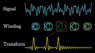
Next, let's explore Fourier Series. Who can define what it does?
It breaks down periodic functions into sine and cosine components.
Exactly! We can represent a function on an interval, like [-L, L], by using a Fourier series. How do we calculate the coefficients a_n and b_n?
We integrate the function times sine or cosine functions over the interval.
Yes! Let's remember 'C.O.E.'—Coefficients, Orthogonality, Expansion. How would we apply Fourier Series to solve PDEs with boundary conditions?
We use sine series for Dirichlet BCs and cosine series for Neumann BCs.
Fantastic summarization! Fourier Series are integral in forming solutions for various initial and boundary conditions. Any remaining questions?
Applications in Civil Engineering
🔒 Unlock Audio Lesson
Sign up and enroll to listen to this audio lesson
Let's connect our knowledge to practical applications. Can anyone think of how these methods apply in civil engineering?
They’re used in heat transfer analysis for structures!
And for analyzing vibrations in beams.
Exactly! These methods allow us to assess critical parameters such as temperature distribution and stress. Remember, these mathematical frameworks are the backbone of our engineering models.
So, it's crucial we understand how to apply these theories effectively?
Absolutely! As civil engineers, mastering these techniques is crucial for designing stable and efficient structures. Let's summarize everything we've learned today.
Introduction & Overview
Read summaries of the section's main ideas at different levels of detail.
Quick Overview
Standard
The separation of variables method simplifies the solution of partial differential equations (PDEs) into ordinary differential equations (ODEs). Coupled with Fourier Series, it allows the expression of complex boundary conditions through infinite sums of sine and cosine functions, crucial for civil engineering applications including heat conduction, fluid flow, and vibration analysis.
Detailed
Detailed Summary
In this section, we delve into two critical mathematical techniques used to solve partial differential equations (PDEs)—the Method of Separation of Variables and Fourier Series.
1. Introduction to PDEs
Partial differential equations arise in the modelling of physical phenomena such as heat transfer, fluid dynamics, and wave propagation. Essential to civil engineering, we categorize these equations as:
- Elliptic (e.g., Laplace's equation for steady-state heat distribution)
- Parabolic (e.g., heat equation for time-dependent heat conduction)
- Hyperbolic (e.g., wave equation for structural vibrations).
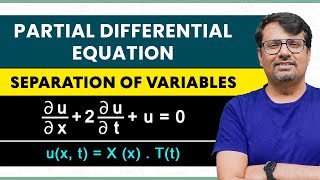
2. Separation of Variables Method
The Separation of Variables technique assumes a solution can be expressed as the product of functions, each dependent on a single variable. The approach involves:
- Substituting the assumed solution into the PDE,
- Separating variables to yield simpler ODEs,
- Applying boundary conditions to solve for constants and eigenfunctions,
- Constructing a general solution with the principle of superposition.
3. Application of Fourier Series
Fourier Series aids in representing a periodic function as a sum of sine and cosine terms, essential for satisfying boundary conditions in PDEs. We differentiate between Fourier Sine Series and Cosine Series based on boundary conditions (Dirichlet and Neumann conditions).
4. Civil Engineering Applications
The techniques discussed are paramount in various civil engineering scenarios, such as:
- Heat Distribution in Structures
- Wave Propagation Analysis
- Fluid Flow Dynamics
- Stress Analysis in Elastic Media.
5. Summary of Key Points
The combination of Separation of Variables and Fourier Series is a potent method for tackling linear PDEs with homogeneous boundary conditions, allowing engineers to express complex phenomena in manageable mathematical terms.
Youtube Videos
Audio Book
Dive deep into the subject with an immersive audiobook experience.
Introduction to Partial Differential Equations (PDEs)
Chapter 1 of 6
🔒 Unlock Audio Chapter
Sign up and enroll to access the full audio experience
Chapter Content
In Civil Engineering, the analysis of structures, heat conduction, fluid flow, and wave propagation often leads to solving partial differential equations (PDEs). A powerful analytical technique for solving linear PDEs is the Method of Separation of Variables combined with the Fourier Series for expressing complex boundary or initial conditions.
Detailed Explanation
This chunk introduces partial differential equations, which are equations that involve rates of change with respect to multiple variables. Engineers often encounter PDEs when dealing with phenomena such as heat transfer or the behavior of structures under stress. The Method of Separation of Variables provides a systematic approach to simplify these equations into ordinary differential equations (ODEs). Understanding this concept is crucial for applying mathematical tools to real-world engineering problems.
Examples & Analogies
Think of a chef trying to bake a cake with a complex recipe. Instead of making the entire cake in one go, the chef might focus on mixing the batter first (one part of the recipe) and then focusing on the frosting separately (another part). Similarly, separation of variables allows engineers to tackle each variable in a problem independently, making complex calculations more manageable.
Types of Partial Differential Equations
Chapter 2 of 6
🔒 Unlock Audio Chapter
Sign up and enroll to access the full audio experience
Chapter Content
The three classical types of second-order PDEs relevant to civil engineering problems are:
- Elliptic PDEs: e.g., Laplace’s equation, for steady-state heat distribution or potential flow.
- Parabolic PDEs: e.g., Heat equation, for time-dependent heat conduction problems.
- Hyperbolic PDEs: e.g., Wave equation, for vibration of structures or wave propagation.
Detailed Explanation
PDEs can be categorized into three main types based on their applications and mathematical properties: Elliptic, Parabolic, and Hyperbolic. Elliptic PDEs often deal with equilibrium situations, like the distribution of heat in a static object. Parabolic PDEs are used for transient phenomena—like how heat spreads over time. Hyperbolic PDEs typically model dynamic systems, such as sound waves or vibrations in beams.
Examples & Analogies
Imagine you are standing in a still pond (an elliptic scenario) and throwing a pebble into the water. The ripples created in the water represent hyperbolic phenomena, while how the water eventually settles down relates to parabolic conditions. This analogy illustrates how different types of PDEs are critical for understanding various physical situations.
Method of Separation of Variables Procedure
Chapter 3 of 6
🔒 Unlock Audio Chapter
Sign up and enroll to access the full audio experience
Chapter Content
The Separation of Variables method assumes the solution of a PDE can be written as the product of single-variable functions. This method is applicable to linear PDEs with homogeneous boundary conditions.
General Procedure:
1. Assume a solution of the form:
u(x,t)=X(x)T(t)
2. Substitute into the PDE.
3. Separate the equation such that each side depends on only one variable:
1/dT = -λ/T(t) = 1/d2X/X(x)
where λ is the separation constant.
4. Solve the resulting ODEs:
- One in x
- One in t
5. Apply boundary conditions to determine allowed values of λ and corresponding eigenfunctions.
6. Construct the general solution as a series using the principle of superposition.
Detailed Explanation
The step-by-step procedure described here outlines how to apply the separation of variables method. By assuming that a solution can be expressed as a product of functions, we can simplify the original PDE into two ODEs. Each of these can be solved independently, allowing the application of boundary conditions to find specific solutions. The separation constant λ plays a crucial role in determining the form of the solution.
Examples & Analogies
Consider solving a puzzle where the overall picture consists of several smaller pieces. Each piece can be viewed as an independent image. In our method, we are isolating each piece (or variable) to examine them closely before combining them into the complete image (solution of the PDE).
Example: Solving the One-Dimensional Heat Equation
Chapter 4 of 6
🔒 Unlock Audio Chapter
Sign up and enroll to access the full audio experience
Chapter Content
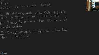
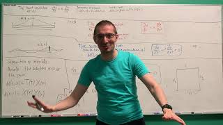
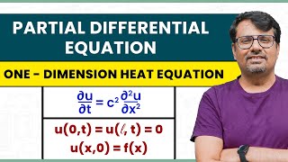
The heat equation in one dimension is:
∂u/∂t = α² ∂²u/∂x²
with conditions:
- u(0,t)=u(L,t)=0 (boundary conditions)
- u(x,0)=f(x) (initial condition)
Step 1: Assume solution
u(x,t)=X(x)T(t)
Step 2: Substitute into PDE
X(x) = α²T(t)
Step 3: Solve ODEs
- Temporal ODE: dT/dt + α²λT = 0, T(t) = Ce−α²λt
- Spatial ODE: d²X/dx² + λX = 0
- Applying boundary conditions X(0)=X(L)=0 leads to: X(x)=sin(nπx/L), λ=(nπ/L)²
Step 4: General solution
∞
u(x,t)=Σ Cₙsin(nπx/L)e−α²(nπ/L)²t (n=1 to ∞)
Detailed Explanation
This example illustrates how to solve a specific PDE using the separation of variables method. The heat equation describes how heat distributes over time through a rod with certain boundary conditions. By assuming the solution can be expressed as a product of spatial and temporal functions and substituting these into the equation, we derive two ODEs. Solving each yields a series solution, which satisfactorily meets both the initial and boundary conditions.
Examples & Analogies
Imagine you’re monitoring the temperature in a long metal rod. The equation helps you predict how heat moves through it over time, much like how the weather forecast predicts temperature changes. By breaking down the complex interactions of heat into manageable parts, engineers can make accurate predictions about thermal behavior.
Fourier Series Overview
Chapter 5 of 6
🔒 Unlock Audio Chapter
Sign up and enroll to access the full audio experience
Chapter Content
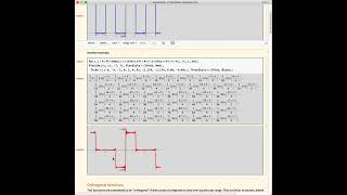
A Fourier series represents a periodic function f(x) as a sum of sines and cosines.
For a piecewise continuous function f(x) on [−L,L]:
∞
f(x) = a₀/2 + Σ (aₙ cos(nπx/L) + bₙ sin(nπx/L))
(n=1 to ∞)
Where coefficients are:
- a₀ = 1/(2L) ∫[−L]L f(x)dx
- aₙ = 1/L ∫[−L]L f(x)cos(nπx/L)dx
- bₙ = 1/L ∫[−L]L f(x)sin(nπx/L)dx
Detailed Explanation
A Fourier series allows us to express complicated periodic functions as sums of simpler sine and cosine functions. This is useful because these are basic building blocks of cyclic behavior. The coefficients a₀, aₙ, and bₙ are derived through integration, ensuring that the series accurately represents the original function over a specific interval. This transformation is fundamental in solving PDEs with non-simple boundary conditions.
Examples & Analogies
Imagine an orchestra playing music. Each instrument contributes its sound (like sine and cosine functions) to create a full symphony (the original function). By separating the parts, you can focus on each instrument to understand how they all come together to form a harmonious piece. This is how Fourier series function—the instruments are the sine and cosine components that create complex periodic functions.
Applications of Fourier Series in PDE Solutions
Chapter 6 of 6
🔒 Unlock Audio Chapter
Sign up and enroll to access the full audio experience
Chapter Content
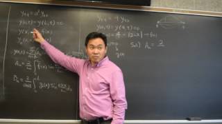
Once the eigenfunctions from the separation of variables are found (usually sine or cosine terms), the unknown coefficients Cₙ are determined using the initial condition via Fourier expansion:
Cₙ = (2/L) ∫[0]L f(x)sin(nπx/L)dx
This allows expressing any arbitrary initial state (e.g., temperature distribution) as a weighted sum of the eigenfunctions.
Detailed Explanation
This chunk explains how the Fourier series is applied once we find the eigenfunctions using separation of variables. The coefficients Cₙ represent how much of each sine function is needed to recreate the initial state of the problem, like a recipe adjusting the quantity of ingredients to achieve the desired final dish. This technique enables us to express complex initial conditions as simple series, offering insights into system behavior.
Examples & Analogies
Think about baking a cake again, where each ingredient (flour, sugar, eggs) must be added in the right amounts. Similarly, the coefficients in the Fourier series determine how much of each sine function contributes to the overall solution. By tuning these amounts, you can perfectly model the initial temperature or displacement in a system.
Key Concepts
-
Separation of Variables: A technique to simplify PDEs into ODEs.
-
Fourier Series: A representation of a periodic function as a sum of sine and cosine terms.
-
Orthogonality: Eigenfunctions are orthogonal, meaning they provide a structurally rich basis for function representation.
Examples & Applications
For the one-dimensional heat equation, u(x,t) can be expressed using Fourier sine series representing the initial temperature distribution.
In analyzing a vibrating beam, the displacement can be modeled using the wave equation with Fourier series representing boundary conditions.
Memory Aids
Interactive tools to help you remember key concepts
Rhymes
For heat flow where states are steady, Laplace's guides, make math-ready.
Stories
Once upon a time, a wise engineer faced challenges in heat transfer. He discovered that by separating variables, he could turn complex problems into manageable equations, using Fourier's magic to represent boundaries with sine and cosine.
Memory Tools
To remember the separation method, think 'S.O.L.V.E.': Substitute, ODEs, Lambda, Values, Eigenfunctions.
Acronyms
P.E.H. P stands for PDEs, E for Elliptic, H for Heat conduction; helps recall problem types!
Flash Cards
Glossary
- Partial Differential Equation (PDE)
An equation involving partial derivatives of a function of multiple variables.
- Eigenfunction
A function that has a specific property of being scaled by an eigenvalue when operated on by a linear operator.
- Fourier Series
A way to represent a function as an infinite sum of sine and cosine functions.
- Orthogonality
A concept in linear algebra where functions are orthogonal if their inner product is zero.
Reference links
Supplementary resources to enhance your learning experience.