
Use in Fluid Flow – Laplace’s Equation
Enroll to start learning
You’ve not yet enrolled in this course. Please enroll for free to listen to audio lessons, classroom podcasts and take practice test.
Interactive Audio Lesson
Listen to a student-teacher conversation explaining the topic in a relatable way.
Introduction to Laplace's Equation in Fluid Flow
🔒 Unlock Audio Lesson
Sign up and enroll to listen to this audio lesson

Today, we're going to explore Laplace's equation, which is critical for modeling fluid flow in civil engineering. Can anyone tell me what Laplace's equation looks like?

Is it the equation that looks like the second derivatives added together to equal zero?
Exactly! It's expressed as ∂²ϕ/∂x² + ∂²ϕ/∂y² = 0. This equation helps us understand the potential flow in fluid mechanics. Now, can someone explain why we would want to use this equation?

I think it's because it helps us find how fluids behave under certain conditions, right?
Correct! Laplace’s equation helps describe phenomena such as potential flow over dams or weirs. Now, remember the acronym CALM, which stands for 'Computational Algorithms for Laplace Modeling'.
Separation of Variables Method
🔒 Unlock Audio Lesson
Sign up and enroll to listen to this audio lesson

Let’s now delve into how we can simplify Laplace's equation using the separation of variables. Who can tell me what we mean by separation of variables?

It's when we assume that the solution can be broken down into functions of single variables!
That's right! We set ϕ(x, y) = X(x)Y(y) and substitute this into the equation. After substitution, we can separate the equation so that one side only depends on x and the other only on y. Can anyone explain what we do next?

We solve the ordinary differential equations that we get from separating the variables!
Absolutely! And applying appropriate boundary conditions after solving these ODEs gives us the potential function we need. Don't forget the mnemonic, 'SIMPLE' – Solve Individual Multipliers and Potential Laplace Equations. Great job!
Boundary Conditions in Fluid Flow Applications
🔒 Unlock Audio Lesson
Sign up and enroll to listen to this audio lesson
Boundary conditions are crucial when solving fluid flow problems using Laplace's equation. Can someone explain what kind of boundary conditions we might encounter?
We could have specified head at a boundary or no-flow conditions at certain walls!
Exactly! Specified head conditions give us the potential at the boundary, while no-flow or Neumann conditions imply that there is no gradient across that wall. Can anyone think of an example in civil engineering?
Like flow under sheet piles?
Yes! Great example. Flow under sheet piles often needs consideration of no-flow conditions on the impermeable walls. Make sure you remember this when modeling. Use the acronym BARRIER – Boundary Analysis Represents Relevant Inflow Edges and Regions.
Practical Applications of Laplace’s Equation
🔒 Unlock Audio Lesson
Sign up and enroll to listen to this audio lesson
Finally, let's discuss practical applications. Can anyone mention where Laplace's equation is used in engineering?
It's used for potential flow analysis over various structures!
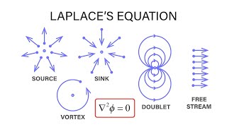
Absolutely! It's prominent in designs involving dams, weirs, and other hydraulic structures. As you think about these applications, remember the acronym FLOW – Fluid’s Laws Over Waters.
Does this apply to situations where we look at groundwater flow too?
Great question! Yes, groundwater flow analysis is a significant application as well. Always connect theory with practice!
Introduction & Overview
Read summaries of the section's main ideas at different levels of detail.
Quick Overview
Standard
The section discusses Laplace's equation in two dimensions, detailing how separation of variables is utilized to solve fluid flow problems with various boundary conditions. It highlights the significance of boundary shape and type in applying this method effectively.
Detailed
Use in Fluid Flow – Laplace’s Equation
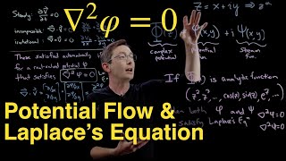
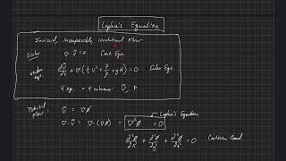
Laplace’s equation plays a critical role in understanding fluid flow conditions, particularly in scenarios like potential flow over structures (e.g., dams or weirs) and flow under barriers such as sheet piles. It is given by the expression:
$$\frac{\partial^2 \phi}{\partial x^2} + \frac{\partial^2 \phi}{\partial y^2} = 0$$
In solving this equation, separation of variables can provide solutions under the condition that the boundary shape is rectangular. The method assumes the solution can be expressed as a product of functions of single variables, denoting the potential function as:
$$\phi(x, y) = X(x)Y(y)$$
Substituting this into Laplace’s equation transforms it into separate ordinary differential equations that can be solved individually for each variable. The boundary conditions need to align with the physical setup and may include specific values like head at a boundary or defining no-flow conditions (Neumann boundary conditions) on impermeable walls. Using Fourier series, one can meet these boundary conditions effectively, ensuring accurate modeling of various fluid flow scenarios in engineering applications.
Youtube Videos

Audio Book
Dive deep into the subject with an immersive audiobook experience.
Introduction to Laplace’s Equation in Fluid Flow
Chapter 1 of 4
🔒 Unlock Audio Chapter
Sign up and enroll to access the full audio experience
Chapter Content
Laplace’s Equation in 2D:
∂²ϕ / ∂x² + ∂²ϕ / ∂y² = 0
Detailed Explanation
Laplace's equation is a second-order partial differential equation that describes how a scalar potential function ϕ varies in a two-dimensional space. It is commonly used in fluid dynamics, particularly in situations where the flow is steady and incompressible. This equation can be interpreted as stating that the sum of the second derivatives of ϕ with respect to both x and y is equal to zero, which indicates there are no local maxima or minima—points of equilibrium—in the flow.
In simpler terms, when we solve the Laplace equation, we are looking for the potential function ϕ that best describes how fluid flows in a given area, such as around or over obstacles.
Examples & Analogies
Imagine a calm pond. The surface of the water represents the potential function ϕ. If we drop a smooth stone in the pond, waves spread out uniformly across the surface, following paths dictated by the boundaries of the pond (the edges of our area of interest). The calm areas—and how far the ripples go—can be thought of as solutions to Laplace's equation in our 2D plane.
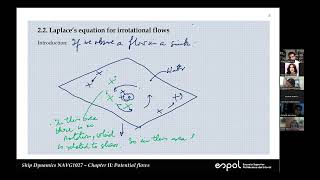
Boundary Conditions and Their Importance
Chapter 2 of 4
🔒 Unlock Audio Chapter
Sign up and enroll to access the full audio experience
Chapter Content
Boundary Conditions depend on geometry:
• Potential flow over dam, weir
• Flow under sheet piles
Detailed Explanation
Boundary conditions are constraints necessary to solve partial differential equations like Laplace's equation. They define how the potential function behaves at the edges of the domain we’re investigating. For instance, one common scenario is potential flow over a dam or weir, where we might specify a certain potential value at the water surface. Alternatively, for flow under sheet piles, we may use a 'no-flow' condition, indicating that fluid cannot penetrate through the wall formed by the sheet piles. These conditions are essential for obtaining a unique solution to the equation and depend heavily on the specific physical situation being modeled.
Examples & Analogies
Think of boundary conditions like the rules in a game. Just as rules dictate how players can behave in a game, boundary conditions set the limits on how fluid can behave at the edges of the area we’re studying. If you're playing soccer and there’s a wall around the field, the wall is a boundary condition that restricts where the ball can go—just like how the conditions around our domain restrict how the fluid flows.
Application of Separation of Variables
Chapter 3 of 4
🔒 Unlock Audio Chapter
Sign up and enroll to access the full audio experience
Chapter Content
Separation of Variables works if boundary is rectangular: Assume ϕ(x,y)=X(x)Y(y), solve ODEs accordingly.
Detailed Explanation
The method of separation of variables is a powerful analytical technique used to solve partial differential equations like Laplace’s equation. This method assumes that the potential function can be expressed as the product of two separate functions: one that depends only on x (X(x)) and another that depends only on y (Y(y)). This makes it easier to solve because we can break down the problem into simpler ordinary differential equations (ODEs) for each variable. If the boundaries are rectangular, this approach can be straightforwardly applied, leading to more manageable calculations and solutions.
Examples & Analogies
Imagine trying to bake a cake where the recipe calls for mixing flour and water separately before combining them. Instead of tackling the entire cake-making process at once (solving the PDE), you first work with just flour (X(x)) and then with water (Y(y)). Once you’ve mixed them perfectly, combining the two yields a delicious cake (the final solution). This analogy highlights the efficiency of breaking problems into parts when dealing with complex tasks.
Use of Fourier Series for Boundary Conditions
Chapter 4 of 4
🔒 Unlock Audio Chapter
Sign up and enroll to access the full audio experience
Chapter Content
Fourier sine/cosine series then help satisfy conditions like:
• Specified head on boundary
• No-flow (Neumann) conditions on impermeable walls
Detailed Explanation
Once the solutions for X(x) and Y(y) are obtained using the method of separation of variables, Fourier series are employed to satisfy the boundary conditions. Fourier sine and cosine series allow for the representation of complex boundary behaviors by decomposing functions into simpler sine and cosine terms. For example, if we need a specific head (height of fluid) at the boundary, we can use a Fourier series to construct a function that meets this requirement. Similarly, a Fourier cosine series can be used to model no-flow conditions at impermeable walls, ensuring that the potential function behaves correctly at those boundaries.
Examples & Analogies
Consider composing music. Just as you can break down a complex melody into individual notes (sine and cosine terms), the Fourier technique lets you piece together boundary conditions from simpler components. If you want your music to follow a particular beat (the boundary conditions), you can tweak the individual notes until they create the desired tune, just like adjusting the Fourier components to achieve the proper flow behavior at the edges of your fluid domain.
Key Concepts
-
Laplace's Equation: Governs potential flow and steady states in fluid dynamics.
-
Separation of Variables: Method for breaking down Laplace's equation into simpler parts.
-
Boundary Conditions: Essential for solving differential equations, specific to the problem's constraints.
Examples & Applications
The flow of water behind a dam can be modeled using Laplace's equation to predict potential distribution.
Analyzing groundwater flow beneath a levee or sheet pile wall using no flow boundary conditions.
Memory Aids
Interactive tools to help you remember key concepts
Rhymes
For flow in a dam, Laplace we won't scram, boundaries defined, but variables combined.
Stories
Picture a serene lake behind a sturdy dam. The only flow is the gentle kiss of wind as water glimmers, all controlled by invisible lines of potential defined by Laplace’s equation.
Memory Tools
Remember 'FLUID' for Fluid Laws Under Incompressible Dynamics indicating Laplace's foundational role.
Acronyms
Use 'BASIC' to recall Boundary Analysis, Separation of variables, and Important conditions.
Flash Cards
Glossary
- Laplace’s Equation
A second-order partial differential equation that describes the potential fields, including fluid flow under steady conditions.
- Separation of Variables
A mathematical method used to simplify partial differential equations by expressing the solution as a product of functions of single variables.
- Boundary Conditions
Conditions defined at the boundaries of a domain that the solution of a differential equation must satisfy.
- Neumann Boundary Conditions
Boundary conditions that specify the derivative of a function on a boundary, often indicating no flow across impermeable walls.
- Potential Flow
Flow where the fluid velocity is derived from a potential function, applicable to irrotational flow conditions.
Reference links
Supplementary resources to enhance your learning experience.