
Method of Separation of Variables
Enroll to start learning
You’ve not yet enrolled in this course. Please enroll for free to listen to audio lessons, classroom podcasts and take practice test.
Interactive Audio Lesson
Listen to a student-teacher conversation explaining the topic in a relatable way.
Introduction to Separation of Variables
🔒 Unlock Audio Lesson
Sign up and enroll to listen to this audio lesson

Today, we start with the Method of Separation of Variables! This method is pivotal in solving partial differential equations by assuming that we can express our solution as a product of functions, each depending on a single variable. Can anyone tell me why this might be useful?

I think it simplifies complex equations into simpler ones?
Excellent point, Student_1! By separating variables, we reduce a PDE to simpler ordinary differential equations, making them much easier to solve. This is especially useful in engineering applications.

Could you give an example of what kind of equations we’re dealing with?
Certainly! A common equation is the heat equation, which describes how heat diffuses through a medium. We can apply the separation method here to analyze it. Let's break down the steps involved in this process.
Steps in the Method
🔒 Unlock Audio Lesson
Sign up and enroll to listen to this audio lesson

Now that we understand the concept, let's walk through the steps of applying the Separation of Variables. Step 1: Assume a solution of the form: u(x, t) = X(x)T(t). Why do we start with this assumption?

It’s to break the solution into parts we can handle separately!
Exactly! Next, we substitute this into our PDE, which leads us to Step 3: separating the equation so that each component is dependent on only one variable. This separation introduces a constant, λ.

What does λ represent, and how important is it?
Good question, Student_4! λ is called the separation constant, and it helps us derive eigenfunctions during the solution process. By finding the values of λ, we can identify the valid temperature or spatial distributions.
Solving ODEs and Boundary Conditions
🔒 Unlock Audio Lesson
Sign up and enroll to listen to this audio lesson
After separation, we have two ordinary differential equations to solve, one for X(x) and one for T(t). Anyone remember why boundary conditions are critical at this step?
They allow us to determine the specific solutions that fit our physical situation… like the edges of a conduction problem?
Exactly! By applying the boundary conditions, we can compute discrete values for λ and obtain corresponding eigenfunctions. This helps us construct our complete solution, often represented as a series.
So, this series can give us an infinite number of solutions that align with the initial conditions?
Precisely! This characteristic makes Fourier series so powerful in practical applications.
Applications of the Method
🔒 Unlock Audio Lesson
Sign up and enroll to listen to this audio lesson
Let’s connect all the dots by discussing real-world applications. The separation of variables method is not just theoretical; it greatly impacts civil engineering, particularly in heat transfer and vibration analysis. Can anyone provide a specific application?
How about temperature distribution in structures?
Yes! Finding temperature distribution in walls or beams based on initial conditions is a direct application. As you see, this method informs design decisions and simulations in engineering.
And I guess it must also help in other areas like fluid flow and wave propagation?
Exactly right. These principles form the cornerstones of various analyses in engineering fields!
Introduction & Overview
Read summaries of the section's main ideas at different levels of detail.
Quick Overview
Standard
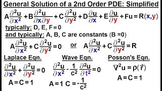
This method involves expressing the solution of linear PDEs as a product of functions, each dependent on a single variable. It is particularly useful with homogeneous boundary conditions, helping to separate the variables and transform the PDE into simpler ordinary differential equations (ODEs) for which solutions can be constructed.
Detailed
Method of Separation of Variables
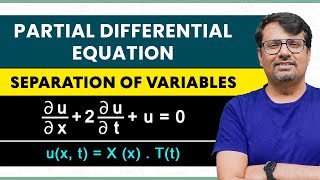
The Method of Separation of Variables is a powerful mathematical technique often used in the analysis of partial differential equations (PDEs), particularly in fields like civil engineering. In this method, the assumption is made that the solution of a PDE can be represented as the product of single-variable functions. This separation allows for simplifying complex PDEs into manageable ordinary differential equations (ODEs). The steps to implement this method include:
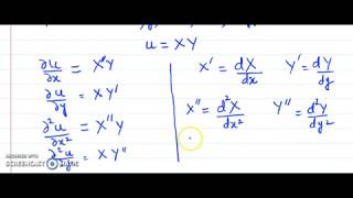
- Assuming a solution of the form:
$$u(x, t) = X(x)T(t)$$ - Substituting this assumed solution into the PDE.
- Separating the resulting equation such that each side depends solely on one variable, leading to the introduction of a separation constant (λ).
- Solving the resulting ODEs individually for both spatial (X) and temporal (T) components.
- Applying boundary conditions to extract discrete eigenvalues and eigenfunctions.
- Constructing a general solution as a series through the principle of superposition, allowing for complex initial or boundary conditions to be satisfied through the use of Fourier series.
Overall, this method streamlines the solving of PDEs while also establishing a broader framework for using Fourier series, which further express complex functions relevant to specific problems.
Youtube Videos
Audio Book
Dive deep into the subject with an immersive audiobook experience.
Introduction to Separation of Variables
Chapter 1 of 4
🔒 Unlock Audio Chapter
Sign up and enroll to access the full audio experience
Chapter Content
The Separation of Variables method assumes the solution of a PDE can be written as the product of single-variable functions. This method is applicable to linear PDEs with homogeneous boundary conditions.
Detailed Explanation
The Separation of Variables technique is a mathematical method used to solve partial differential equations (PDEs). It operates on the principle that a complex problem can be simplified by splitting the variables involved. Specifically, it assumes that the solution can be represented as a product of separate functions, each depending on a single variable. This is particularly useful for linear PDEs under certain conditions known as homogeneous boundary conditions, where the solution behaves predictably at the boundaries of the domain.
Examples & Analogies
Think of this method like baking a cake. Instead of making one big batter, you can treat the wet and dry ingredients separately. First, mix all the dry ingredients and then all the wet ones. Finally, combine them to make the cake. Similarly, in Separation of Variables, we handle each part of the problem separately to make it easier to find the solution.
General Procedure of Separation of Variables
Chapter 2 of 4
🔒 Unlock Audio Chapter
Sign up and enroll to access the full audio experience
Chapter Content
General Procedure:
1. Assume a solution of the form:
u(x,t)=X(x)T(t)
2. Substitute into the PDE.
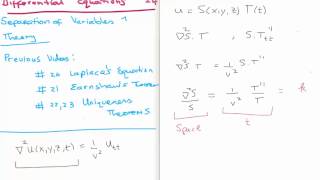
3. Separate the equation such that each side depends on only one variable:
1 dT 1 d2X
= =−λ
T(t) dt X(x) dx2
• where λ is the separation constant.
4. Solve the resulting ODEs:
• One in x
• One in t
5. Apply boundary conditions to determine allowed values of λ and corresponding eigenfunctions.
6. Construct the general solution as a series using the principle of super-position.
Detailed Explanation
The Separation of Variables method follows a systematic approach:
1. It begins by assuming a solution in the form of a product of functions, one spatial (X) and the other temporal (T).
2. After substituting this assumed solution into the original PDE, the method separates the dependent variables so that one side of the equation depends only on time, while the other depends solely on space.
3. This process introduces a constant, λ, known as the separation constant, which helps to further simplify the problem.
4. The next step involves solving these separate ordinary differential equations (ODEs) for both X and T.
5. Boundary conditions are then applied to find permissible values of λ, which correspond to specific solutions or eigenfunctions.
6. Finally, the general solution is constructed using a series, employing the principle of superposition, which allows for the summation of multiple eigenfunctions to form a complete solution.
Examples & Analogies
Imagine you want to find out how a swing moves in both time and space. First, you could think of the motion of the swing as two separate things: how high it goes (related to time) and where it is in the yard (related to space). By treating each aspect separately and then piecing them together, it becomes much easier to predict the overall swinging motion—just as the Separation of Variables method breaks down complex equations into manageable parts.
Solving the Resulting ODEs
Chapter 3 of 4
🔒 Unlock Audio Chapter
Sign up and enroll to access the full audio experience
Chapter Content
- Apply boundary conditions to determine allowed values of λ and corresponding eigenfunctions.
Detailed Explanation
After solving for X(x) and T(t) from the separated equations, we apply specific conditions known as boundary conditions. These conditions arise from the physical scenario being modeled and help in determining the specific solutions to the equations. By solving for allowed values of the separation constant λ, we can find corresponding functions called eigenfunctions that satisfy both the differential equations and the boundary conditions set by the problem.
Examples & Analogies
Think about hitting a target with an arrow. The position of the target relates to where you can aim your arrow (boundary conditions), and the type of arrows you have (values of λ) affects how accurately you can hit the target. By understanding the dynamics of both the target and the arrows, you can effectively figure out how to hit the target.
Constructing the General Solution
Chapter 4 of 4
🔒 Unlock Audio Chapter
Sign up and enroll to access the full audio experience
Chapter Content
- Construct the general solution as a series using the principle of superposition.
Detailed Explanation
Using the solutions for X(x) and T(t) derived from the previous steps, we combine these solutions to form a general solution. This is done through a method called superposition, which states that the overall effect (in this case, the solution to the PDE) can be expressed as the sum of simpler effects (the individual solutions). This approach allows for creating a series of solutions that can effectively address the complexity of the original PDE.
Examples & Analogies
Think of a music symphony where several instruments play together. Each instrument represents a specific solution, and when played together, they create a beautiful piece of music—much like how combining different solutions creates the overall solution to a PDE.
Key Concepts
-
Separation of Variables: A method to transform PDEs into ODEs by assuming solutions can be expressed as products of single-variable functions.
-
Eigenfunctions: The functions derived from the spatial ODEs which lead to the solution's general form.
-
Boundary Conditions: Constraints applied to determine specific solutions relevant to physical situations.
Examples & Applications
The heat equation, used in determining temperature distribution in a concrete slab over time.
The wave equation, which describes vibrations or waves within a given medium, applicable in structural engineering.
Memory Aids
Interactive tools to help you remember key concepts
Rhymes
When solving PDEs, don’t despair, / Separate the variables, if you dare!
Stories
Imagine a chef who can combine ingredients to make different dishes. Just like the chef uses different ingredients, the method of separation allows us to combine functions to create solutions for complex equations.
Memory Tools
S → Separate, A → Apply, S → Solve, C → Construct (SASC) - remember the key steps!
Acronyms
SEPARATE
Solve Equations by Partial Analysis in Reduced And Transformed Equations.
Flash Cards
Glossary
- Partial Differential Equation (PDE)
An equation involving partial derivatives of a multivariable function.
- Ordinary Differential Equation (ODE)
An equation involving functions of a single variable and their derivatives.
- Eigenfunction
A function that remains unchanged except for a scalar factor when an operator is applied to it.
- Separation Constant (λ)
A constant that arises when separating variables in a PDE, aiding in the solution process.
- Fourier Series
A way to represent a function as an infinite sum of sines and cosines.
Reference links
Supplementary resources to enhance your learning experience.