
Heat Equation Animation (Conceptual)
Enroll to start learning
You’ve not yet enrolled in this course. Please enroll for free to listen to audio lessons, classroom podcasts and take practice test.
Interactive Audio Lesson
Listen to a student-teacher conversation explaining the topic in a relatable way.
Understanding the Heat Equation
🔒 Unlock Audio Lesson
Sign up and enroll to listen to this audio lesson

Today, we're going to learn about the heat equation and how we can visualize its solutions over time. Can anyone remind me what the heat equation fundamentally describes?

It describes how heat diffuses through a material over time.
Exactly! So, at time `t=0`, we have our initial distribution of temperatures represented by `f(x)`. What do you think happens to this temperature distribution as time increases?

I think the temperature starts to change and spread out.
Good observation! As time goes on, higher frequency components, or rapid temperature fluctuations, begin to die out faster, leaving us with mostly lower frequency components.

So eventually, only the slower changes remain?
Exactly! This leads to a more uniform temperature across our medium. Let's visualize this in our upcoming animation.
Visualizing Mode Dominance
🔒 Unlock Audio Lesson
Sign up and enroll to listen to this audio lesson

Now, let’s delve into the animation. As time progresses, you'll see how fast temperature waves dissipate. Can anyone tell me what’s meant by ‘higher frequency components’ in this context?

They are the rapid changes in temperature, like sharp increases or decreases.
Right! And those tend to vanish more quickly compared to the low-frequency components. Why do you think that's important in real-world applications?
It helps engineers to understand how materials will respond to heat over time.
Absolutely! As we work with structures, it’s crucial to know how heat will distribute and stabilize. Let’s look at the animation to get a clearer picture.
Conclusion and Real-World Implications
🔒 Unlock Audio Lesson
Sign up and enroll to listen to this audio lesson
As we wrap up our discussion on heat conduction, can someone summarize what we learned about the patterns of temperature distribution?
We learned that at the start, the temperature distribution is defined by the initial condition, and over time, higher frequencies fade out, stabilizing the temperature.
Well said! And why is this behavior significant for civil engineering?
It shows us how structures might react to temperature changes, helping in designing better and safer buildings.
Exactly! Understanding this concept is essential for effective thermal management in structural engineering. Thank you, everyone!
Introduction & Overview
Read summaries of the section's main ideas at different levels of detail.
Quick Overview
Standard
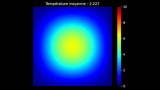
The heat equation animation illustrates how temperature distribution changes from an initial state over time, emphasizing the diminishing impact of higher frequency components as the system approaches steady state with only lower frequency modes present.
Detailed
Heat Equation Animation (Conceptual)
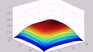
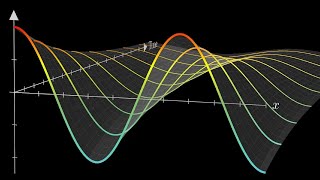
The heat equation describes how heat diffuses through a medium over time. This section visualizes the process through an animation depicting various stages in the evolution of temperature distribution.
- Initial Condition: At time
t=0, the temperature distribution is fully defined by a functionf(x), which represents the initial temperature at different points in the medium. - Progression Over Time: As time progresses, the influence of higher frequency components of the solution diminishes more rapidly compared to lower frequency ones. This results in the system gradually stabilizing towards a steady-state solution, where only long-wavelength (low-frequency) modes dominate the temperature distribution.
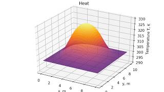
- Significance: This phenomenon reflects how high-frequency variations in temperature (rapid fluctuations) are smoothed out, leading to a more stable and uniform temperature in the medium over time. The visualization emphasizes the importance of understanding heat conduction in engineering and design applications, as it informs how structures will respond to thermal loads.
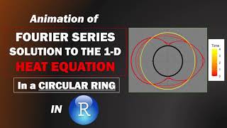
Youtube Videos


Audio Book
Dive deep into the subject with an immersive audiobook experience.
Initial Temperature Distribution
Chapter 1 of 3
🔒 Unlock Audio Chapter
Sign up and enroll to access the full audio experience
Chapter Content
• At t=0: Temperature is fully described by f(x)
Detailed Explanation
At the start of the observation (t=0), the temperature profile of the material is determined solely by the function f(x). This function f(x) illustrates how temperature varies along the length of the material at that specific moment in time. Essentially, it gives us a snapshot of the heat distribution throughout the object before any time has elapsed.
Examples & Analogies
Imagine a loaf of bread just out of the oven. The temperature of the bread varies at different points—it may be hottest in the center and cooler on the edges. The function f(x) represents this initial temperature distribution right when you take the bread out. Just like you'd feel those temperature differences as you touch various parts of the loaf, f(x) characterizes how heat is distributed from the beginning.
Evolution of Temperature Over Time
Chapter 2 of 3
🔒 Unlock Audio Chapter
Sign up and enroll to access the full audio experience
Chapter Content
• As t increases: Higher frequency components die out faster
Detailed Explanation
As time progresses, the temperature dynamics change. The higher frequency components in the temperature distribution tend to dissipate more rapidly than lower frequency components. In simpler terms, the sharp fluctuations or rapid changes in temperature (high frequencies) will disappear faster than the more gradual changes (low frequencies). This reflects a natural smoothing process wherein asymmetric heat distributions tend to even out over time.
Examples & Analogies
Think of a crowded room where a party is taking place. Initially, the energy (or 'temperature') might fluctuate wildly with lots of excitement in one area (high frequencies) and quieter zones. As time passes, people start to mingle and energy levels even out, with fewer extreme highs and lows in energy (low frequencies). Just like the room's atmosphere, the initial sharp temperature differences start to blend and smooth out over time.
Dominance of Low-Frequency Modes
Chapter 3 of 3
🔒 Unlock Audio Chapter
Sign up and enroll to access the full audio experience
Chapter Content
• Eventually: Only low-frequency modes (longer wavelengths) dominate
Detailed Explanation
In the long run, as the system stabilizes, it becomes dominated by low-frequency temperature modes characterized by longer wavelengths. This means that the temperature distribution in the material becomes smoother and more uniform, resembling the overall average state of the system. These low-frequency modes are often associated with the more gradual, slow-moving changes in heat distribution rather than rapid fluctuations.
Examples & Analogies
Consider a lake with ripples on the surface after you drop a stone into it. Initially, many small ripples (high frequencies) spread out quickly and are very pronounced. However, over time, these ripples fade, leaving behind a calm surface (low frequency). Eventually, the lake appears smooth, representing a uniform average state. This is similar to how the heat distribution in the material settles into a steady state dominated by low-frequency modes.
Key Concepts
-
Initial Temperature Distribution: The state of temperature in the medium at time
t=0as given by the functionf(x). -
Diminishing Higher Frequency Components: Over time, higher frequency components in the temperature distribution decrease more rapidly than lower frequency components.
-
Steady State: The eventual uniform temperature distribution achieved as fluctuations die out and only low-frequency modes remain.
Examples & Applications
If a metal rod is heated on one end, the immediate temperature distribution can be described using an initial function. As time progresses, the sharp temperature changes will diminish.
In a heating process of a building, initial temperature differences between rooms will equalize over time as described by the principles of the heat equation.
Memory Aids
Interactive tools to help you remember key concepts
Rhymes
Heat travels slow, fast changes go. As time does flow, steady state we know!
Stories
Once upon a time, in a land of temperature, there were fast and slow changes. As the sun rose, the fast changes ran away, leaving only the steady and calm, low changes behind.
Memory Tools
SLOW: Steady, Low-frequencies Over time dominate.
Acronyms
HEAT
High-frequency components Escape After Time passes.
Flash Cards
Glossary
- Heat Equation
A partial differential equation that describes the distribution of heat in a given region over time.
- Initial Condition
The temperature distribution at the initial time
t = 0in the context of a heat problem.
- Frequency Components
Sine and cosine components of a Fourier series representation, indicating different modes of variation in the function.
- LowFrequency Modes
Components of a solution that represent slow variations and dominate the behavior as time progresses.
Reference links
Supplementary resources to enhance your learning experience.