
Non-Homogeneous Systems
Enroll to start learning
You’ve not yet enrolled in this course. Please enroll for free to listen to audio lessons, classroom podcasts and take practice test.
Interactive Audio Lesson
Listen to a student-teacher conversation explaining the topic in a relatable way.
Understanding Non-Homogeneous Systems
🔒 Unlock Audio Lesson
Sign up and enroll to listen to this audio lesson

Today we are going to discuss non-homogeneous systems. Can someone tell me what a non-homogeneous system looks like?

Is it where the right-hand side is not zero, like in Ax = b when b ≠ 0?
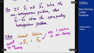
Exactly! In a non-homogeneous system, the presence of a non-zero b indicates that solutions are displaced from the origin. The general solution combines a particular solution with solutions to the corresponding homogeneous system.

So, how do we actually find the general solution?
That's a great question! If we find a particular solution, we can express the complete solution as x = xp + xh, where xp is the particular solution and xh is the solution to the homogeneous system Ax = 0. Remember the acronym P + H: Particular plus Homogeneous equals General!

Can you give an example of how this works?
Certainly! If we determine a particular solution, we would then find the null space of A to identify xh. Putting it together gives us the full picture.
Solving Non-Homogeneous Systems
🔒 Unlock Audio Lesson
Sign up and enroll to listen to this audio lesson

Now, let’s discuss the method of actually solving these systems. What do we start with?

We begin with finding a particular solution, right?
Correct! After identifying a particular solution, we move on to solve the homogeneous part. Can someone remind me what the homogeneous equation looks like?
It’s Ax = 0, the same matrix without the b vector!
Spot on! And remember, every solution to our non-homogeneous system can be represented as a linear combination of our found particular and homogeneous solutions.
Does that mean we can have infinitely many solutions for non-homogeneous systems too?
Yes! If the homogeneous system has more than just the trivial solution, then the non-homogeneous system will also have infinitely many solutions.
Application of Non-Homogeneous Solutions
🔒 Unlock Audio Lesson
Sign up and enroll to listen to this audio lesson
Let’s talk about where these systems appear in practical scenarios. Can anyone think of a situation or field where non-homogeneous systems might be used?
Maybe in engineering when analyzing forces?
Exactly! In engineering, non-homogeneous systems can model various real-world phenomena where offsets or external forces act on a structure or system. Understanding how to derive the solutions helps ensure stability and safety.
Do we use numeric methods or algorithms to solve these systems in practice?
Absolutely! Numerical methods, like LU decomposition or iterative algorithms, are often employed in computing environments when dealing with larger systems.
So mastering these concepts is vital for future work in engineering?
Yes, indeed! The more comfortable you become with these methods, the more proficient you will be in applying them effectively.
Introduction & Overview
Read summaries of the section's main ideas at different levels of detail.
Quick Overview
Standard
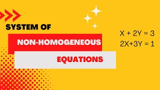
This section discusses non-homogeneous systems of linear equations, highlighting how they differ from homogeneous systems. A non-homogeneous system consists of equations that include a non-zero constant, and its general solution is formed by adding a particular solution to the solutions of the associated homogeneous system.
Detailed
In this section, we explore non-homogeneous systems of linear equations, defined by the equation Ax = b, where b ≠ 0. The main highlight is that if there exists a particular solution (denoted as xp), the complete set of solutions can be constructed by adding this particular solution to the solutions of the corresponding homogeneous system, Ax = 0. The general solution can thus be expressed as x = xp + xh, where xh lies in the null space of A. This understanding is crucial as it illustrates how solutions to a system can be systematically related to one another, thereby providing a deeper insight into the problem-solving process in linear algebra.
Youtube Videos

![[Linear Algebra] Nonhomogeneous System Solutions](https://img.youtube.com/vi/axkmcrVdQPc/mqdefault.jpg)

Audio Book
Dive deep into the subject with an immersive audiobook experience.
General Solution of Non-Homogeneous Systems
Chapter 1 of 2
🔒 Unlock Audio Chapter
Sign up and enroll to access the full audio experience
Chapter Content
For b≠0, if a particular solution x_p exists, then the general solution is given by:
x = x_p + x_h
Where:
- x_p: A particular solution.
- x_h: General solution of the homogeneous system Ax=0.
Detailed Explanation
In this section, we explore non-homogeneous systems, which are systems of equations where the constant term (often represented as b) is not equal to zero. Non-homogeneous systems can often be solved if we know at least one solution (referred to as x_p). The general solution of such systems expresses every possible solution as a combination of this particular solution and the solutions of the related homogeneous system (where b equals zero). Since each homogeneous system has its own solutions (x_h), adding these to the particular solution gives us a complete set of solutions for the non-homogeneous system.
Examples & Analogies
Imagine you're trying to find all the routes to a school (the general solution) but you already know one route that you can take (the particular solution, x_p). The school is not just at that route (since b≠0 represents the necessary conditions). Now consider all the other possible routes that form the roads (the homogeneous solutions, x_h). By combining the known route with all other possible roads, you map out every route to the school.
Meaning of Each Component in the General Solution
Chapter 2 of 2
🔒 Unlock Audio Chapter
Sign up and enroll to access the full audio experience
Chapter Content
This means every solution of the non-homogeneous system is a sum of one particular solution and all solutions of the associated homogeneous system.
Detailed Explanation
In more detail, the general solution's structure allows us to understand how we can find solutions to complex systems of equations. The idea is that the solution to the non-homogeneous part (where b is not zero) builds directly off of the known solutions from the homogeneous case. Anything added to the known solution that fulfills the restrictions of the homogeneous system still serves as a valid solution for the entire scenario. This structural relationship shows the beauty and neatness of how linear systems can be solved systematically.
Examples & Analogies
Think of solving non-homogeneous systems like baking a cake (non-homogeneous) where you already have the base recipe (the homogeneous solution). The particular cake you've already baked is one version (x_p), while the base recipe allows you to add various toppings or adjustments (the general solutions, x_h) to create different delicious cakes from the same base recipe.
Key Concepts
-
Non-Homogeneous Systems: Systems characterized by an equation set with a non-zero constant on the right side.
-
Particular Solution: A specific solution to a non-homogeneous system that satisfies the given equations.
-
Homogeneous System: A system where the equations equal zero, allowing exploration of solutions without external influences.
-
General Solution: The solution representation that combines particular and homogeneous solutions.
-
Null Space: The vector subspace containing all solutions to the homogeneous equation.
Examples & Applications
The equation system 2x + 3y = 5 and x - y = 1 represents a non-homogeneous system with a simple solution set.
In civil engineering, determining the equilibrium of forces often leads to solving non-homogeneous systems to ensure structure stability.
Memory Aids
Interactive tools to help you remember key concepts
Rhymes
For non-homogeneous, don’t be shy, b is key and can’t be dry!
Stories
Imagine a group of friends (solutions) sitting apart (non-homogeneous). They still feel connected through the center of their meeting spot (particular solution). Together, they form a lively gathering spanned by their unique places!
Memory Tools
P + H = G helps to remember that Particular + Homogeneous gives General solution.
Acronyms
NHP
Non-Homogeneous Problem to remind you of unique challenges in systems with distinct solutions.
Flash Cards
Glossary
- NonHomogeneous System
A system of linear equations where the right-hand side vector b is not equal to zero.
- Particular Solution
A specific solution to a non-homogeneous system that satisfies Ax = b.
- Homogeneous System
A system of linear equations where the right-hand side vector is zero, represented as Ax = 0.
- General Solution
The complete set of solutions to a system which combines a particular solution and the solutions of the corresponding homogeneous system.
- Null Space
The set of all solutions to the homogeneous equation Ax = 0.
Reference links
Supplementary resources to enhance your learning experience.