
Rank Deficiency and Least Squares Approximation
Enroll to start learning
You’ve not yet enrolled in this course. Please enroll for free to listen to audio lessons, classroom podcasts and take practice test.
Interactive Audio Lesson
Listen to a student-teacher conversation explaining the topic in a relatable way.
Overdetermined Systems
🔒 Unlock Audio Lesson
Sign up and enroll to listen to this audio lesson

Let's begin by discussing what an overdetermined system is. Can anyone tell me what happens in such systems?

Is it when you have more equations than unknowns?
Exactly! In an overdetermined system, where we have many equations but fewer unknowns, we can encounter inconsistencies. That means there may not be a solution that satisfies all the equations simultaneously. This is where we need least squares approximation. Can anyone explain what a least squares approach does?

It tries to minimize the error between the equations and the solutions?
Right! It minimizes the square of the norm of the differences between the actual and predicted values, mathematically expressed as \(\min \|Ax - b\|_2^2\).

So, it's like finding the best fit for the data we have?
Yes, exactly! Now, for practical scenarios, why is it important to minimize the error in this way?

Because in real-world applications, our measurements and data may not align perfectly.
Absolutely! That's fundamental in fields like civil engineering when analyzing data to create models.
To summarize, in overdetermined systems, we may not have 'exact' solutions due to inconsistencies, and least squares allows us to find the best approximate solution.
Formulation of the Least Squares Problem
🔒 Unlock Audio Lesson
Sign up and enroll to listen to this audio lesson

Now let’s break down how we can formally set up the least squares problem. Does anyone remember how we begin this process?
We set up the equation system to minimize?
Correct! We start with \(Ax = b\) and aim to minimize \(\|Ax - b\|_2^2\). Now, how can we express this in matrix form?
By multiplying both sides with the transpose of A?
Exactly! We get the normal equation: \(A^TAx = A^Tb\). Can anyone explain what \(A^TA\) represents in terms of the matrix?
It's a symmetric matrix, right?
Yes! And this step is crucial in ensuring that we can solve for x. What do you think is the advantage of using this approach in applications?
It gives us a clear method to find an estimate even when the system is inconsistent.
Exactly! And this is essential in fields like civil surveying and calibration of sensor networks. In summary, by applying the least squares approximation, we can effectively manage situations where our system of equations fails to be consistent.
Pseudo-Inverse in Solutions
🔒 Unlock Audio Lesson
Sign up and enroll to listen to this audio lesson
Lastly, let’s discuss the pseudo-inverse. Who remembers what the pseudo-inverse does?
Is it used when A isn't square or when it's not invertible?
Exactly! For non-square or rank-deficient matrices, we can define the pseudo-inverse \(A^+\) to calculate solutions. How does that look mathematically?
It's \(x = A^+b\).
Great! Now can anyone provide an example of where we might use this concept in real life?
In sensor network calibration, if we have readings that don't perfectly match up.
Exactly! The pseudo-inverse enables us to still obtain a meaningful solution despite the system's deficiencies. To wrap up this session, the pseudo-inverse is crucial for handling cases where traditional methods fail, particularly in modern applications involving sensor data.
Introduction & Overview
Read summaries of the section's main ideas at different levels of detail.
Quick Overview
Standard
The section explores how overdetermined systems can lead to inconsistencies and how the least squares approach minimizes the error in solutions. It covers the formulation of least squares problems and the role of the pseudo-inverse in obtaining solutions for non-square or rank-deficient matrices.
Detailed
Rank Deficiency and Least Squares Approximation
This section focuses on understanding the problem of rank deficiency in linear systems, particularly in the context of overdetermined systems, where the number of equations (m) exceeds the number of unknowns (n). Due to this situation, such systems may lead to inconsistencies between equations. Consequently, it is critical to seek a solution that minimizes the error in the least squares sense, defined mathematically as minimizing the norm of the residual:
$$\min \|Ax - b\|_2^2$$
Any optimal solution, if achievable, can be obtained by solving the equation:
$$A^TAx = A^Tb$$
This approach is fundamental in various applications such as civil surveying, curve fitting, and sensor calibration, where obtaining an approximate solution is vital despite the potential inconsistency present in data. Additionally, the concept of the pseudo-inverse (Moore-Penrose) is introduced for cases where the matrix A is not square or invertible, allowing the calculation of:
$$x = A^+b$$
This segment emphasizes the utility of least squares approximation in practical scenarios where traditional solutions may not be feasible.
Youtube Videos


Audio Book
Dive deep into the subject with an immersive audiobook experience.
Overdetermined Systems
Chapter 1 of 2
🔒 Unlock Audio Chapter
Sign up and enroll to access the full audio experience
Chapter Content
When m>n, the system may be inconsistent. In such cases, we seek a solution that minimizes the error in a least squares sense:
min∥Ax−b∥²
The solution is given by:
AT Ax=ATb
Used in:
- Civil surveying.
- Curve fitting in construction data.
- Sensor network calibration.
Detailed Explanation
In this section, we discuss overdetermined systems, which occur when there are more equations (m) than unknowns (n). These systems might not have an exact solution due to inconsistency among the equations. Therefore, we look for solutions that minimize the error between the left and right sides of the equation. The term ‘least squares’ refers to the method of minimizing the sum of the squares of the residuals (the differences between observed and predicted values). The mathematical expression for this minimization is represented as 'min∥Ax−b∥²', where 'x' is the solution vector we are trying to find. The equation 'AT Ax=ATb' provides the least squares solution for this problem, helping us estimate the best possible fit for our data even when exact solutions are not feasible.
Examples & Analogies
Imagine you are trying to find the best possible path to connect several cities for a new highway. You gather data from various routes taken by other vehicles, but there may not be a single path that connects all cities perfectly without conflict. By applying least squares approximation, you analyze all the data to determine a route that minimizes the overall traveling distance, even if it doesn't perfectly connect every city along the way. This route may be seen as a compromise that provides the best fit for the urban landscape.
Pseudo-Inverse (Moore-Penrose)
Chapter 2 of 2
🔒 Unlock Audio Chapter
Sign up and enroll to access the full audio experience
Chapter Content
If A is not square or not invertible:
x=A⁺b
Where A⁺ is the pseudo-inverse of A.
Detailed Explanation
The pseudo-inverse, or Moore-Penrose inverse, is a generalization of the inverse matrix that can be applied to non-square or singular matrices, which have no conventional inverse. When a matrix 'A' is either not square (more equations than unknowns) or not invertible (det(A)=0), we can still attempt to find a solution 'x' using the pseudo-inverse. The relationship is given by 'x=A⁺b', where 'A⁺' represents the pseudo-inverse of 'A'. This allows us to find a solution that minimizes the residual error, similar to the least squares method discussed earlier, providing important flexibility in solving linear systems.
Examples & Analogies
Think of trying to fit a square peg into a round hole. If the peg (matrix A) is not the right shape or size, you can't fit it exactly. However, if you allow for some adjustments — like reshaping the peg or the hole — you can still find a way to connect them. The pseudo-inverse acts like this adjustment, allowing you to find a solution that fits the requirements as closely as possible, even when a perfect fit isn’t achievable.
Key Concepts
-
Overdetermined Systems: These systems have more equations than unknowns, leading to potential inconsistencies.
-
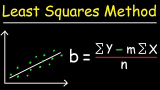
Least Squares Method: This technique is used to minimize discrepancies in overdetermined systems.
-
Pseudo-Inverse: It provides a way to solve linear systems when the standard inverse cannot be applied, especially for rank-deficient matrices.
Examples & Applications
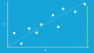
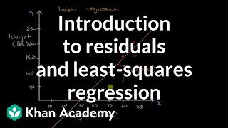
Example of curve fitting using least squares, where a data set does not match a linear equation perfectly.
Example of applying the pseudo-inverse in sensor calibration, where not all sensor readings align, but an approximate solution is required.
Memory Aids
Interactive tools to help you remember key concepts
Rhymes
With many lines and just one aim, least squares will ease the fitting game.
Stories
Imagine a data analyst trying to fit a curve to messy data with too many points; instead of forcing an answer, they smartly use least squares for the best fit.
Memory Tools
LSE - Least Squares Estimate: Always recall that we estimate using least squares.
Acronyms
OES - Overdetermined Equations Solved
reminder of how least squares helps us solve more equations than unknowns.
Flash Cards
Glossary
- Overdetermined System
A system of equations with more equations than unknowns, possibly leading to inconsistencies.
- Least Squares Approximation
A method of finding an approximate solution that minimizes the sum of the squares of the residuals.
- Normal Equation
The equation \(A^TAx = A^Tb\) used to solve least squares problems.
- PseudoInverse
A generalization of the matrix inverse for non-square or singular matrices, denoted as \(A^+\).
Reference links
Supplementary resources to enhance your learning experience.