
Analyze System Responses in Transient and Steady-State Conditions
Enroll to start learning
You’ve not yet enrolled in this course. Please enroll for free to listen to audio lessons, classroom podcasts and take practice test.
Interactive Audio Lesson
Listen to a student-teacher conversation explaining the topic in a relatable way.
Introduction to System Responses
🔒 Unlock Audio Lesson
Sign up and enroll to listen to this audio lesson

Today, we're diving into an essential topic: system responses, which help us understand how systems behave under different inputs.

What do we mean by 'system response'?
Great question! System responses can be categorized into two main types: transient and steady-state responses. The transient response occurs immediately after a change and reflects how quickly the system reacts.

And what about steady-state response?
The steady-state response is the behavior of the system after it has settled down. It's crucial for understanding overall stability and accuracy.

So, both responses are important for system design?
Exactly! A good design minimizes errors and meets performance criteria.

Can you give us an example?
Sure! If a car's cruise control needs to maintain a speed, understanding both how fast it responds to speed changes and how accurately it maintains that speed is vital.
In summary, we need to analyze both the transient and steady-state responses to create efficient control systems.
Transient Response Characteristics
🔒 Unlock Audio Lesson
Sign up and enroll to listen to this audio lesson

Now let's explore transient response characteristics: rise time, settling time, overshoot, and damping ratio. First, what do you think rise time is?
Is it the time it takes to get to a certain value?
Exactly! It's the time taken for the output to rise from 10% to 90% of its final value.
And what about settling time?
Settling time is the time it takes for the output to stay within a specific range, like 2% or 5%, of its final value. It's an indicator of system stability.
How does overshoot come into this?
Good question! Overshoot refers to how much the output exceeds its steady-state value before settling down, expressed as a percentage of that value.
What impacts these values?
The damping ratio plays a role; it describes the amount of damping in the system, affecting how quickly and smoothly it responds to changes.
To summarize, transient response elements such as rise time, settling time, and overshoot guide us in evaluating system performance.
Steady-State Response Analysis
🔒 Unlock Audio Lesson
Sign up and enroll to listen to this audio lesson
Now that we've covered transient response, let's shift our focus to steady-state response. Who can tell me what steady-state error means?
Is it the difference between what we want and what we actually get?
Correct! It's the difference as time approaches infinity, after transient effects have subsided.
Are there different types of inputs we should consider?
Yes, steady-state error depends on the type of input: step inputs, ramp inputs, and parabolic inputs.
What about error constants? How do they come into play?
Error constants—Kp, Kv, and Ka—help quantify the steady-state error for each input type. Kp pertains to step inputs, Kv for ramps, and Ka for parabolic inputs.
Could you show examples for these constants?
Certainly! For instance, for a step input, the steady-state error can be calculated using the formula: ess = 1 / (1 + Kp).
In summary, steady-state analysis allows us to assess system performance in real-world applications, using error constants tailored to specific inputs.
Introduction & Overview
Read summaries of the section's main ideas at different levels of detail.
Quick Overview
Standard
In this section, we explore the transient and steady-state responses of control systems, focusing on essential parameters like rise time, settling time, and steady-state error. Understanding these responses is crucial for assessing stability and performance in engineering applications.
Detailed
Analyze System Responses in Transient and Steady-State Conditions
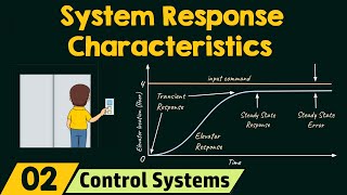
Understanding system responses in transient and steady-state conditions is vital for designing and evaluating control systems. Control systems experience two phases of response:
- Transient Response: Describes how the output behaves immediately following a change in input, such as a step input. Key features include:
- Rise Time (trt): Time taken for output to reach 90% of final value.
- Settling Time (tst): Time required for the output to remain within a certain percentage of its final value.
- Overshoot (Mp): Maximum output exceeding the steady-state value, expressed as a percentage.
- Peak Time (tpt): Time taken to reach the first peak of the response.
- Damping Ratio (ζ) and Natural Frequency (ωn): Both influence the system's response characteristics, including oscillations and settling time.
- Steady-State Response: Describes the system's behavior after it has settled down, focusing on:
- Steady-State Error: Difference between desired and actual output when transient effects fade away, varying with input signal types (step, ramp, parabolic).
- Error Constants: Such as Position (Kp), Velocity (Kv), and Acceleration constants (Ka) provide insights into error characteristics during different input types.
The section emphasizes the importance of both transient and steady-state responses for designing stable and high-performance control systems.
Youtube Videos


Audio Book
Dive deep into the subject with an immersive audiobook experience.
Introduction to System Responses
Chapter 1 of 7
🔒 Unlock Audio Chapter
Sign up and enroll to access the full audio experience
Chapter Content
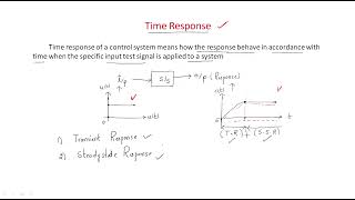
In control systems, understanding the system response is essential to designing stable and high-performance systems. A system's response can be divided into two primary phases:
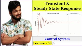
1. Transient Response: The behavior of the system immediately after a change in input (such as a step input) before it reaches steady-state. It reflects how the system reacts to initial disturbances and how quickly it settles to its final value.
2. Steady-State Response: The behavior of the system after it has had enough time to settle and reach equilibrium. It reflects how the system behaves once transient effects have subsided.
Both responses are important for assessing system stability, speed, and accuracy.
Detailed Explanation
This introduction outlines the two critical phases in which any control system's output can be analyzed. The Transient Response happens right after an input change, like a sudden spike in demand or a shift in temperature. It’s about how quickly and effectively the system reacts to these changes. In contrast, the Steady-State Response focuses on the system's behavior after the initial chaos has settled, allowing it to achieve a consistent state. Understanding both of these phases is crucial for ensuring that the system operates reliably and efficiently in practical applications.
Examples & Analogies
Consider a car accelerating. When the driver presses the gas pedal, the initial speed increase corresponds to the Transient Response. How quickly the car accelerates is related to the system's transient characteristics. Once the car reaches a constant speed and maintains that speed on the highway, it reflects the Steady-State Response. Understanding how quickly the car responds to the driver's command and how it maintains speed matters for safe driving.
Understanding Transient Response
Chapter 2 of 7
🔒 Unlock Audio Chapter
Sign up and enroll to access the full audio experience
Chapter Content
The transient response of a system describes how the output behaves immediately after a change in the input, such as a sudden step, ramp, or impulse input. It is characterized by the following features:
1. Rise Time (trt_r): The time it takes for the output to go from 10% to 90% of its final value. It indicates how quickly the system responds to changes.
2. Settling Time (tst_s): The time required for the output to stay within a certain percentage (e.g., 2% or 5%) of its final value. It provides an indication of how long the system takes to stabilize after a disturbance.
3. Overshoot (MpM_p): The maximum peak value of the output response, expressed as a percentage of the steady-state value. Overshoot reflects how much the system exceeds the desired output before settling down.
4. Peak Time (tpt_p): The time it takes for the system to reach the first peak of its response.
5. Damping Ratio (ζ): A dimensionless measure that describes the amount of damping in the system. It influences the speed and overshoot of the transient response. Systems with higher damping have less oscillation and faster settling times.
6. Natural Frequency (ωn): The frequency at which the system oscillates in the absence of damping. It is related to the speed of the transient response.
Detailed Explanation
The transient response reveals how the system behaves right after an input change, which is critical in many applications. Features like Rise Time and Settling Time help define how fast the system can react and stabilize, respectively. Overshoot describes any temporary spike in the output, which can be crucial for applications where precise control is necessary, like in robotics or aerospace. Damping Ratio affects oscillation and stability; a higher ratio means that the system will settle faster and with less fluctuation, impacting overall performance. Natural Frequency indicates how quickly the system can respond to changes, which is vital for design.
Examples & Analogies
Imagine pouring a glass of water: when you first pour it, water rushes in (the transient response). How quickly it fills to near full (rise time) and how long it takes to settle without spilling (settling time) are critical. If you pour too quickly, it might overflow (overshoot). The water's behavior is influenced by how smoothly you pour (damping), just like how a controlled system behaves.
Mathematical Representation of Transient Response
Chapter 3 of 7
🔒 Unlock Audio Chapter
Sign up and enroll to access the full audio experience
Chapter Content
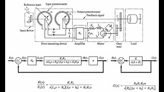
For a second-order system, the transfer function is given by:
G(s)=ωn² / (s² + 2ζωns + ωn²)
The system's time-domain response to a step input (using the inverse Laplace transform) is given by:
y(t)=1−1/√(1−ζ²)e^(−ζωnt)sin(ω_d t + ϕ)
where:
● ωd=ωn√(1−ζ²) is the damped natural frequency.
● ϕ=arccos(ζ) is the phase angle.
Detailed Explanation
The equations provided represent a mathematical way to predict the behavior of the system during its transient response. The transfer function shows how the output of the system relates to its input in frequency terms. The time-domain response equation illustrates how the system will respond over time after a sudden change in input, considering factors like damping and frequency, which shape the oscillatory behavior of the system.
Examples & Analogies
Think of a swing being pushed. The transfer function corresponds to how much you push and how far the swing goes. The time-domain equation captures the swing's motion as it goes back and forth (oscillation) until it eventually comes to rest. The timing of these oscillations can be modeled mathematically to predict how the swing will behave.
Effects of Damping on Transient Response
Chapter 4 of 7
🔒 Unlock Audio Chapter
Sign up and enroll to access the full audio experience
Chapter Content
● Underdamped (0<ζ<1): The system exhibits oscillations that decay over time.
● Critically damped (ζ=1): The system returns to steady-state without oscillating, but as fast as possible.
● Overdamped (ζ>1): The system returns to steady-state slowly without oscillating.
Detailed Explanation
Damping plays a significant role in how the transient response is characterized. In the case of underdamping, the system oscillates around the steady-state value, leading to potential overshoot. Critical damping allows the system to settle quickly without excess oscillation, which is ideal for many engineering applications. Overdamping results in a slow return to steady-state, which might be undesirable for systems that require quick responses.
Examples & Analogies
Imagine a trampoline. When you bounce (underdamped), you go up and down before settling down. If it’s set perfectly (critically damped), you come to rest quickly without bouncing. If it’s too stiff (overdamped), it just sinks slowly onto the ground, taking longer to settle down.
Steady-State Response Overview
Chapter 5 of 7
🔒 Unlock Audio Chapter
Sign up and enroll to access the full audio experience
Chapter Content
Once the system has settled and transient effects have subsided, the system reaches a steady-state. The steady-state response describes how the output behaves in response to a constant input after the transient effects die out. Key factors in analyzing steady-state response include:
1. Steady-State Error: The difference between the desired output and the actual output as time approaches infinity.
2. Error Constants: These are used to determine the steady-state error for different types of inputs: Step input, ramp input, or parabolic input.
Detailed Explanation
The steady-state response is important for assessing how accurately a system can maintain its output once it has stabilized. The steady-state error indicates how far the actual output gets from the desired output, showing if the system is functioning accurately enough for practical use. Error constants help quantify these errors for various types of inputs—these constants directly inform how the system should be designed or adjusted to minimize errors for specific conditions.
Examples & Analogies
Think of a thermostat in a house. When the temperature is set, it works to reach that temperature (steady-state), but if it overshoots or undershoots, the little adjustments it makes indicate the steady-state error. The thermostat continually measures temperature (error constant), trying to settle at the target temperature accurately.
Calculating Steady-State Error
Chapter 6 of 7
🔒 Unlock Audio Chapter
Sign up and enroll to access the full audio experience
Chapter Content
Error Constants:
- Position Error Constant Kp: Determines the steady-state error for a step input.
Kp=lim s→0G(s)H(s) - Velocity Error Constant Kv: Determines the steady-state error for a ramp input.
Kv=lim s→0 s⋅G(s)H(s) - Acceleration Error Constant Ka: Determines the steady-state error for a parabolic input.
Ka=lim s→0 s²⋅G(s)H(s)
Steady-State Error Formulae:
- Step Input: e_ss = 1/(1 + Kp)
- Ramp Input: e_ss = 1/Kv
- Parabolic Input: e_ss = 1/Ka
Detailed Explanation
Error constants define how a system will behave under different input scenarios. By calculating Kp, Kv, and Ka, we gain insight into how the system will respond to step, ramp, or parabolic inputs. The formulas give specific values that describe how much error will occur in a steady state, allowing engineers to predict the system's performance under different operating conditions effectively.
Examples & Analogies
Imagine you’re adjusting the volume on a speaker. The step input is similar to turning the volume up (Kp). If you gradually increase the volume (ramp input), you can measure how quickly it reaches a comfortable level (Kv). For a speaker that can play a smooth audio crescendo (parabolic input), gradually reaching maximum sound, that’s like measuring how well it responds over time to various adjustments (Ka). Each adjustment type corresponds to an error constant that helps you understand how to tune the speaker.
Conclusion of System Responses
Chapter 7 of 7
🔒 Unlock Audio Chapter
Sign up and enroll to access the full audio experience
Chapter Content
In this chapter, we examined both the transient and steady-state responses of control systems. The transient response provides insight into the system's behavior during the transition from one state to another, while the steady-state response describes the system's behavior once it has settled. Engineers use various time-domain and frequency-domain methods to analyze these responses, allowing them to design systems with optimal performance in terms of speed, accuracy, and stability.
Detailed Explanation
This conclusion summarizes the critical concepts of the chapter, emphasizing how transient and steady-state responses are vital for control system analysis. Understanding both types of responses equips engineers and designers to create systems tailored for desired specifications, ensuring they operate effectively within their intended applications. The various analytical methods allow for deeper insights and optimizations based on performance objectives.
Examples & Analogies
Consider a well-designed spacecraft. Engineers must ensure that it can respond quickly to control commands (transient) while also being stable during long missions (steady-state). They apply the principles discussed in this chapter, similarly to mastering the balance between quick maneuvering and stable cruising, ensuring that the spacecraft performs optimally in all landing or orbital situations.
Key Concepts
-
Transient Response: The initial behavior of the system right after an input change.
-
Steady-State Response: The behavior of the system once the effects of transients have diminished.
-
Damping Ratio (ζ): Indicates how oscillations in the system are affected.
Examples & Applications
Example: If a second-order system has a damping ratio of 0.5, it will exhibit oscillations that decay over time.
Example: For a system with Kp = 10, the steady-state error for a step input would be 0.09.
Memory Aids
Interactive tools to help you remember key concepts
Rhymes
For time to elevate, rise without wait—10% to 90%, that's the rise fate.
Stories
Imagine a swing coming to a stop after being pushed. It swings back and forth (overshoot) before finally coming to rest — that's the transient response in action!
Memory Tools
Remember the acronym ROSe (Rise time, Overshoot, Settling time) to keep track of transient response characteristics.
Acronyms
DREAM for Damping, Rise time, Error (steady-state), and Accuracy for system analysis.
Flash Cards
Glossary
- Transient Response
The system behavior immediately following a change in input before reaching steady-state.
- SteadyState Response
The behavior of the system after transient effects have subsided and it reaches equilibrium.
- Rise Time (trt)
The time required for the output to rise from 10% to 90% of its final value.
- Settling Time (tst)
The time taken for the output to remain within a specified value of its final value.
- Overshoot (Mp)
The maximum peak value of the output in excess of the steady-state value.
- Damping Ratio (ζ)
A dimensionless measure that indicates the extent of damping in the system.
- Error Constants
Quantities (Kp, Kv, Ka) that determine the steady-state error for specific input types.
Reference links
Supplementary resources to enhance your learning experience.