
Parabolic input
Enroll to start learning
You’ve not yet enrolled in this course. Please enroll for free to listen to audio lessons, classroom podcasts and take practice test.
Interactive Audio Lesson
Listen to a student-teacher conversation explaining the topic in a relatable way.
Understanding Steady-State Error for Parabolic Input
🔒 Unlock Audio Lesson
Sign up and enroll to listen to this audio lesson

Today, we're going to delve into steady-state errors, especially in relation to parabolic inputs. Can anyone remind me what we mean by steady-state error?

Isn’t it the difference between the desired output and the actual output when the system has settled?
Exactly! Now, the steady-state error (ess) for parabolic inputs is particularly important for analyzing how a system reacts to sustained disturbances. We represent it using the acceleration error constant, K_a.

How do we calculate that steady-state error for parabolic inputs?
Great question! For parabolic inputs, the formula for steady-state error is $$ e_{ss} = \frac{1}{K_a} $$, where K_a signifies the system’s ability to handle acceleration. If K_a is high, the system has a lower steady-state error.

So, if we want to minimize the steady-state error, we need a larger K_a, right?
Absolutely correct! The larger the K_a value, the more robust our system will be in handling parabolic disturbances. This analysis is crucial for ensuring system performance.
Application of Steady-State Error in Control Systems
🔒 Unlock Audio Lesson
Sign up and enroll to listen to this audio lesson

Now that we understand how to calculate steady-state error for parabolic inputs, let’s discuss some real-world applications. What kinds of systems do you think would benefit from a low steady-state error?

I think automated vehicle control systems would need to react accurately to changing speeds.
Exactly! In such systems, the ability to properly handle acceleration, which includes parabolic inputs, is vital for safety. Can anyone think of other applications?
Robotics! They need precise control to follow parabolic paths smoothly.
Spot on! Low steady-state error ensures that robotic movements are accurate and seamless. This reinforces the importance of understanding K_a in control system design.
Introduction & Overview
Read summaries of the section's main ideas at different levels of detail.
Quick Overview
Standard
In control systems, the steady-state error for a parabolic input is explained through the acceleration error constant (Ka). This specific error analysis plays a crucial role in understanding the system's performance in response to sustained parabolic disturbances or inputs.
Detailed
Detailed Summary
The study of steady-state error for different types of input signals is vital in control system analysis. In this section, we focus on the parabolic input, which can be considered a more aggressive and continuous type of disturbance affecting the system response. The steady-state error (ess) for a parabolic input is derived using the acceleration error constant (Ka). The formula for steady-state error when responding to a parabolic input is as follows:
$$ e_{ss} = \frac{1}{K_a} $$
Here, Ka is a measure of the system's capability to handle acceleration-based inputs, quantifying the steady-state error under parabolic conditions. By understanding how this error constant impacts system performance, engineers can design more effective control systems that accurately compensate for varying types of inputs, ensuring improved stability and responsiveness.
Youtube Videos


Audio Book
Dive deep into the subject with an immersive audiobook experience.
Understanding Parabolic Input Response
Chapter 1 of 3
🔒 Unlock Audio Chapter
Sign up and enroll to access the full audio experience
Chapter Content
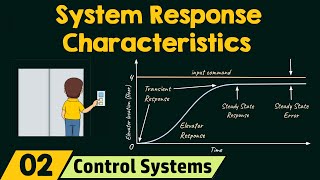
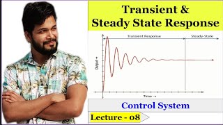
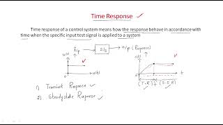
Once the system has settled and transient effects have subsided, the system reaches a steady-state. The steady-state response describes how the output behaves in response to a constant input after the transient effects die out. Key factors in analyzing steady-state response include:
Detailed Explanation
This chunk explains the steady-state response of a system after it has reacted to transient inputs. In simple terms, when we change the input to a control system (like changing the speed of a robot), it takes some time for the system to respond and stabilize. Once it does stabilize, it operates at a steady-state where we can predict how it will behave over time. This is important in analyzing how effectively a system meets its desired performance goals.
Examples & Analogies
Imagine driving a car. When you press on the gas pedal (change in input), the car doesn’t start moving instantly; it takes a moment to gain speed. When the car reaches a constant speed, that’s like the steady-state response. If you maintain your foot on the pedal, the car continues to drive smoothly, just as a control system operates steadily after settling.
Key Factors of Steady-State Response
Chapter 2 of 3
🔒 Unlock Audio Chapter
Sign up and enroll to access the full audio experience
Chapter Content
- Steady-State Error: The difference between the desired output and the actual output as time approaches infinity.
- Error Constants:
- Position Error Constant Kp: Determines the steady-state error for a step input.
- Velocity Error Constant Kv: Determines the steady-state error for a ramp input.
- Acceleration Error Constant Ka: Determines the steady-state error for a parabolic input.
Detailed Explanation
In this chunk, we discuss the factors involved in determining the steady-state response. The steady-state error is critical; it tells us how well the system can achieve the desired output as time goes on. For different types of inputs (like step, ramp, and parabolic), we need specific error constants (Kp, Kv, Ka) to quantify these errors. These constants help us understand how much the system will deviate from the desired outcome.
Examples & Analogies
Think of a child trying to hit a moving target with a dart. If the target moves in a straight line (like a step input), the child can measure how far off they were from hitting it. If the target speeds up steadily (like a ramp input), they would need to adjust their aim based on the speed of the target, and this adjustment relates to the velocity error constant. In each scenario, they learn how effectively they can hit the target based on their practice and adjustments, similar to how control systems adjust to achieve their targets.
Steady-State Error for Different Inputs
Chapter 3 of 3
🔒 Unlock Audio Chapter
Sign up and enroll to access the full audio experience
Chapter Content
Steady-State Error Formulae:
- Step Input: For a system with a transfer function G(s), the steady-state error for a step input R(s) is given by:
ess = 1 / (1 + Kp)
- Ramp Input: The steady-state error for a ramp input R(s) = 1/s^2 is given by:
ess = 1 / Kv
- Parabolic Input: The steady-state error for a parabolic input R(s) = 1/s^3 is given by:
ess = 1 / Ka.
Detailed Explanation
This chunk presents the specific mathematical formulae for calculating the steady-state error based on the type of input provided to the system. For a step input, the formula depends on Kp (position error constant), while for a ramp input it uses Kv (velocity error constant), and for a parabolic input it employs Ka (acceleration error constant). Understanding these formulae is crucial because they allow engineers to predict the system's accuracy in attaining its desired performance.
Examples & Analogies
Consider a person learning to shoot basketballs. If they aim to make a basket from a stationary position (step input), the measure of how far they missed (steady-state error) can be determined using their initial attempts (Kp). If they want to make a moving basket a few feet away at a constant speed (like a ramp), they'll adjust their angle differently, needing another measurement (Kv). Finally, if the basket moves in a parabolic arc, they’ll need a different technique altogether, represented by Ka. Each scenario shows how a person makes adjustments based on different conditions, similar to how error constants in control systems help in adjusting outputs.
Key Concepts
-
Steady-State Error: Key figure indicating how accurately a control system can follow a desired path over time.
-
Parabolic Input: A complex input used to examine systems under more aggressive conditions.
-
Acceleration Error Constant (K_a): Central parameter for analyzing the steady-state response of systems subjected to parabolic inputs.
Examples & Applications
If a control system modeled for a robotic arm exhibits a K_a of 20, then the steady-state error when subjected to a parabolic input would be e_ss = 1/20 = 0.05, indicating high accuracy and performance.
In automotive control systems, a high K_a value would ensure that transient steering adjustments can handle aggressive acceleration without significant steady-state error.
Memory Aids
Interactive tools to help you remember key concepts
Rhymes
When inputs are parabolic and rates still climb, K_a keeps the steady state in its prime.
Stories
Imagine a car on a hilly road (parabolic path), needing exact adjustments. With a high K_a, the driver cruises smoothly without error.
Memory Tools
K_a for a parabolic path: Keep our action accurate.
Acronyms
PEAR
Parabolic Error and Acceleration Response. This helps remember to analyze error when dealing with parabolic inputs.
Flash Cards
Glossary
- SteadyState Error
The difference between the desired output and the actual output of a control system as time approaches infinity.
- Parabolic Input
A continuous input signal that changes at an increasing rate, reflecting a parabolic function over time.
- Acceleration Error Constant (K_a)
A constant that quantifies the steady-state error for a parabolic input and indicates a system's responsiveness to acceleration-based disturbances.
Reference links
Supplementary resources to enhance your learning experience.