
Time Domain Analysis
Enroll to start learning
You’ve not yet enrolled in this course. Please enroll for free to listen to audio lessons, classroom podcasts and take practice test.
Interactive Audio Lesson
Listen to a student-teacher conversation explaining the topic in a relatable way.
Transient Response
🔒 Unlock Audio Lesson
Sign up and enroll to listen to this audio lesson

Let's start with the transient response. Can anyone tell me what it refers to in a control system?

Is it how the system reacts immediately after a change in input?
Yes! The transient response shows how quickly the system reacts and how effectively it stabilizes. Key parameters to remember are rise time, settling time, and overshoot.

What do those terms mean?
Good question! Rise time is the time for the output to reach 90% of its final value, while settling time is how long it takes to stay within a certain range of its final value. Can you think of a memory aid for these terms?

Maybe we can remember 'Rising and Settling - Time's Always Spelling'?
That's creative! It's important to focus on these dynamics since they greatly impact system performance. Let's summarize: the transient response characterizes initial system behavior and includes rise time, settling time, and overshoot.
Damping Ratio and Natural Frequency
🔒 Unlock Audio Lesson
Sign up and enroll to listen to this audio lesson

Now let’s discuss the damping ratio and natural frequency. Who can explain what these terms mean?

Damping ratio measures how much a system oscillates.
Exactly! A higher damping ratio means less oscillation and faster settling times. The natural frequency indicates how fast the system oscillates without damping.
Can you give an example of different damping scenarios?
Sure! Under damped systems (0 < ζ < 1) oscillate before settling. Critically damped systems (ζ = 1) return to steady state without oscillating. Lastly, overdamped systems (ζ > 1) settle slowly without oscillation. Remember: 'Under and Over, settle in the middle for the fastest ride!'
This mnemonic is helpful! So, damping affects how our system behaves over time?
Yes! Understanding damping and frequency helps improve system design based on performance requirements.
Steady-State Response
🔒 Unlock Audio Lesson
Sign up and enroll to listen to this audio lesson
Let’s shift to the steady-state response. What is this phase in a control system?
Is it when the system has settled and reached equilibrium?
Exactly! In steady-state, the system output should ideally match the desired input without any fluctuations. One important metric here is the steady-state error.
How do we calculate steady-state error?
Great question! We use error constants for different input types: the position error constant for a step input, the velocity error constant for a ramp input, and the acceleration constant for a parabolic input. Do you recognize the relationships here?
Yes! Different inputs have different error constants affecting our output.
Exactly! That’s crucial for design. To summarize, in steady-state, we focus on how accurately the system achieves desired outputs and we use steady-state error to measure this.
Introduction & Overview
Read summaries of the section's main ideas at different levels of detail.
Quick Overview
Standard
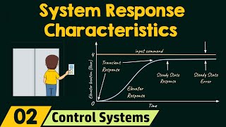
In time domain analysis, the system response is analyzed by evaluating key parameters such as rise time, settling time, and steady-state error. This analysis helps assess how effectively a system reacts and stabilizes after changes in input.
Detailed
Time Domain Analysis
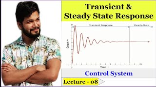
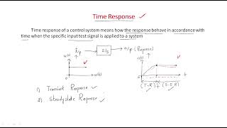
Time domain analysis plays a crucial role in understanding how control systems respond to different inputs over time. This analysis can be categorized into two main responses: transient and steady-state. The transient response assesses the system's behavior immediately after an input change, focusing on parameters such as rise time (how quickly the output reaches its final value), settling time (how long it takes for the output to stabilize within a certain range), overshoot (the extent to which the output exceeds its final value), damping ratio (which affects oscillations), and natural frequency (indicating speed of response).
In contrast, the steady-state response evaluates the long-term behavior of the system after transient effects have diminished. Important metrics include steady-state error, which quantifies the difference between desired and actual output for various inputs like step, ramp, and parabolic inputs. By analyzing both the transient and steady-state responses, engineers can design robust control systems that meet performance specifications.
Youtube Videos


Audio Book
Dive deep into the subject with an immersive audiobook experience.
Evaluating Time-Domain Response
Chapter 1 of 3
🔒 Unlock Audio Chapter
Sign up and enroll to access the full audio experience
Chapter Content
Evaluate the system's time-domain response by solving the system’s differential equations.
Detailed Explanation
The time-domain response of a system describes how the output changes over time in reaction to an input. To analyze this, we use the system's differential equations, which define the relationship between the system's input and output over time. Solving these equations allows us to predict how the system behaves in response to various inputs.
Examples & Analogies
Think of a time-domain response like observing how a car accelerates after you push the gas pedal. The differential equations govern the car's motion, just as they govern a system's output over time.
Common Analytical Techniques
Chapter 2 of 3
🔒 Unlock Audio Chapter
Sign up and enroll to access the full audio experience
Chapter Content
Common techniques include Laplace transforms and inverse Laplace transforms to move between time and frequency domains.
Detailed Explanation
Laplace transforms are a powerful mathematical tool that allows us to convert time-domain functions into frequency-domain representations. This makes it easier to analyze complex systems by simplifying the equations we need to solve. The inverse Laplace transform takes us back to the time domain once we have completed our analysis in the frequency domain.
Examples & Analogies
Imagine using a recipe to prepare a dish. The Laplace transform is like converting the recipe to a healthy version; it simplifies the ingredients and steps. The inverse Laplace transform is like going back to the original recipe after figuring out the new version.
Key Parameters to Analyze
Chapter 3 of 3
🔒 Unlock Audio Chapter
Sign up and enroll to access the full audio experience
Chapter Content
Analyze key parameters like rise time, settling time, overshoot, and steady-state error.
Detailed Explanation
When evaluating a system's time-domain response, specific parameters provide important insights. Rise time indicates how quickly the system responds to changes, settling time shows how long it takes to stabilize, overshoot reflects how much the output exceeds the desired value before settling, and steady-state error tells us the final difference between the desired and actual output in the long term.
Examples & Analogies
Consider a person jumping on a trampoline. Rise time is how fast they get off the trampoline, settling time is how long it takes for them to stop bouncing, overshoot is how high they go above the intended height, and steady-state error is the difference between their highest point and a target height they wanted to reach, like trying to touch a basketball hoop.
Key Concepts
-
Transient Response: The initial reaction of a system to input changes.
-
Rise Time: Time from 10% to 90% of final output.
-
Settling Time: The time to remain within a certain range of the final value.
-
Overshoot: The extent to which the system exceeds its target.
-
Damping Ratio: Affects system oscillation behavior.
-
Natural Frequency: Indicates response speed.
-
Steady-State Response: Behavior when a system stabilizes long-term.
Examples & Applications
For a system with a damping ratio of 0.5 and a natural frequency of 5 rad/s, the response will show oscillations and require specific time to settle.
Calculating steady-state error for a system with a position error constant Kp of 10 yields a steady-state error of 0.09 for a step input.
Memory Aids
Interactive tools to help you remember key concepts
Rhymes
Rise and settle, it’s a race, to find stability in space.
Stories
Imagine a bouncing ball reaching its peak (overshoot), then settling down smoothly — that's akin to our system's journey.
Memory Tools
Remember: 'R.O.S.' for Rise time, Overshoot, and Settling time.
Acronyms
D.A.S.H. - Damping, Amplitude, Settling, Harmonics for key transient concepts.
Flash Cards
Glossary
- Transient Response
The behavior of a system immediately after a change in input before it stabilizes.
- Rise Time
The time taken for the output to rise from 10% to 90% of its final value.
- Settling Time
The duration for the output to remain within a certain percentage of its final value.
- Overshoot
The maximum peak of the output response expressed as a percentage of the final value.
- Damping Ratio
A dimensionless measure of the damping in the system impacting oscillation.
- Natural Frequency
The frequency at which the system oscillates without damping.
- SteadyState Response
The behavior of a system once transient effects have died out.
- SteadyState Error
The difference between the desired output and the actual output as time approaches infinity.
Reference links
Supplementary resources to enhance your learning experience.