
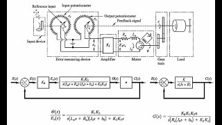
Mathematical Representation
Enroll to start learning
You’ve not yet enrolled in this course. Please enroll for free to listen to audio lessons, classroom podcasts and take practice test.
Interactive Audio Lesson
Listen to a student-teacher conversation explaining the topic in a relatable way.
Transfer Function of a Second-Order System
🔒 Unlock Audio Lesson
Sign up and enroll to listen to this audio lesson

Today, we'll look at the mathematical representation of a second-order system. The transfer function is mathematically expressed as G(s) = ω_n² / (s² + 2ζω_ns + ω_n²). Can anyone tell me the components of this equation?

I think ω_n is the natural frequency, right?
Correct! And what about ζ?

That's the damping ratio, which affects how the system responds.
Exactly! Remember, the damping ratio helps us understand how quickly the system will settle. Both factors are crucial in designing stable systems.
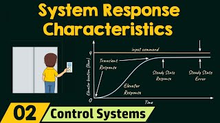
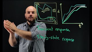
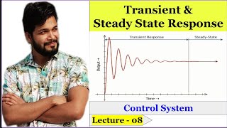
Time-Domain Response to Step Input
🔒 Unlock Audio Lesson
Sign up and enroll to listen to this audio lesson

Now, let's discuss the time-domain response to a step input. The equation is y(t) = 1 - (1/√(1 - ζ²)) e^(-ζω_nt) sin(ω_dt + φ). How do we interpret this?

It looks complex! But I see we have terms that involve ω_d and φ.
Great observation! ω_d represents the damped natural frequency, and φ is the phase angle. These determine the oscillations in the response.

So, if ζ is less than 1, does that mean the system is underdamped?
Exactly, and underdamped systems oscillate before settling. Understanding these responses helps us predict system performance.
Importance of Damping and Natural Frequency
🔒 Unlock Audio Lesson
Sign up and enroll to listen to this audio lesson
Let’s consider the effects of different damping ratios. How do they influence the system?
An underdamped system has oscillations, while a critically damped system returns faster without oscillating.
Correct! An overdamped system reacts the slowest. Why do you think the damping ratio is so crucial?
It helps in tuning system responses to avoid too much overshoot or delay!
Exactly! And the natural frequency indicates how fast the system can respond. Both affect the transient behavior significantly.
Introduction & Overview
Read summaries of the section's main ideas at different levels of detail.
Quick Overview
Standard
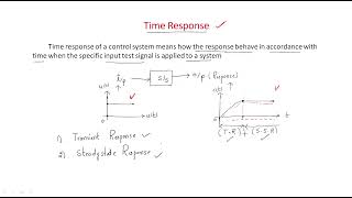
This section provides the mathematical expressions for the transfer function of a second-order system and the time-domain response to a step input. It includes vital parameters like the damping ratio, natural frequency, and their implications for system behavior.
Detailed
Mathematical Representation
The mathematical representation for a second-order system’s transfer function is crucial for understanding its dynamic behavior. The transfer function is given by:
$$ G(s) = \frac{\omega_n^2}{s^2 + 2\zeta \omega_n s + \omega_n^2} $$
In this equation, $\omega_n$ refers to the natural frequency of the system, and $\zeta$ denotes the damping ratio. These parameters critically affect the system's response.
The response to a step input can be found using the inverse Laplace transform:
$$ y(t) = 1 - \frac{1}{\sqrt{1 - \zeta^2}} e^{-\zeta \omega_n t} \sin(\omega_d t + \phi) $$
where:
- $\omega_d = \omega_n \sqrt{1 - \zeta^2}$ is the damped natural frequency.
- $\phi = \arccos(\zeta)$ is the phase angle.
Understanding these equations is pivotal for analyzing how systems behave under various input conditions and aids in designing systems that meet performance specifications.
Youtube Videos

Audio Book
Dive deep into the subject with an immersive audiobook experience.
Transfer Function of a Second-Order System
Chapter 1 of 4
🔒 Unlock Audio Chapter
Sign up and enroll to access the full audio experience
Chapter Content
For a second-order system, the transfer function is given by:
G(s) = \frac{\omega_n^2}{s^2 + 2\zeta\omega_n s + \omega_n^2}
Detailed Explanation
The transfer function describes the relationship between the input and output of a system in the Laplace domain. For a second-order system, it is represented with parameters that include the natural frequency (\omega_n) and the damping ratio (\zeta). This formula is important because it encapsulates how quickly a system responds and how it behaves under different input conditions.
Examples & Analogies
Imagine a swing at a playground. The speed with which it moves (natural frequency) and how much it slows down after being pushed (damping) can be described using a mathematical model similar to this transfer function. By understanding these values, you can predict how high and how quickly the swing will go.
Time-Domain Response to a Step Input
Chapter 2 of 4
🔒 Unlock Audio Chapter
Sign up and enroll to access the full audio experience
Chapter Content
The system's time-domain response to a step input (using the inverse Laplace transform) is given by:
y(t) = 1 - \frac{1}{\sqrt{1 - \zeta^2}} e^{-\zeta\omega_n t} \sin(\omega_d t + \phi)
Detailed Explanation
This equation represents how the output (y(t)) behaves over time when the system receives a sudden change in input, known as a 'step input'. The components include slopes of exponential decay and oscillatory behavior, depending on the damping ratio. It helps us determine how quickly the system reaches its final state and any oscillations around that state.
Examples & Analogies
Consider turning on a water tap for a moment and observing how long it takes for the flow rate to stabilize. At first, it may splutter (the oscillations), but eventually, it settles into a steady stream (the final state). This equation mathematically models that behavior.
Damped Natural Frequency and Phase Angle
Chapter 3 of 4
🔒 Unlock Audio Chapter
Sign up and enroll to access the full audio experience
Chapter Content
where:
● \omega_d = \omega_n \sqrt{1 - \zeta^2} is the damped natural frequency.
● \phi = \arccos(\zeta) is the phase angle.
Detailed Explanation
The damped natural frequency (\omega_d) represents how quickly the system oscillates under damping, showing us that damping changes the effective frequency of oscillation. The phase angle (\phi) determines how the oscillations line up in time, which is crucial for understanding the timing of the response. Together, these parameters allow engineers to predict real-world behavior more accurately.
Examples & Analogies
Think of a team of rowers in a boat. If they all row at the same time, they move forward smoothly (the phase angle aligned). If one rower starts a little late (the phase angle misaligned), the boat wobbles and slows down. The damped frequency would describe how the wobble settles down over time, just like how the rowing technique affects stability.
Effects of Damping on Transient Response
Chapter 4 of 4
🔒 Unlock Audio Chapter
Sign up and enroll to access the full audio experience
Chapter Content
● Underdamped (0 < \zeta < 1): The system exhibits oscillations that decay over time.
● Critically damped (\zeta = 1): The system returns to steady-state without oscillating, but as fast as possible.
● Overdamped (\zeta > 1): The system returns to steady-state slowly without oscillating.
Detailed Explanation
Damping ratio (ζ) affects how a system returns to its final state after a disturbance. In an underdamped system, you see oscillations that gradually decline; in a critically damped system, the response is swift without overshooting; while in an overdamped system, the response is slower and smooth without oscillations. Understanding these behaviors helps engineers design systems according to specific response requirements.
Examples & Analogies
Imagine a car suspension system after hitting a bump. If it doesn’t bounce much before stabilizing, it’s critically damped. If it does bounce a lot before settling down, it’s underdamped. If it slowly settles without bouncing much, it’s overdamped. Each type has its own implications for ride comfort and handling.
Key Concepts
-
Transfer Function: Relationship between input and output in the Laplace domain.
-
Natural Frequency: Determines how fast the system oscillates.
-
Damping Ratio: Influences the decay of oscillations in the transient response.
-
Damped Natural Frequency: Indicates frequency of oscillation in a damped system.
-
Phase Angle: Represents the shift in oscillation timing.
Examples & Applications
For a system with damping ratio ζ = 0.5 and natural frequency ω_n = 5 rad/s, we can derive the transfer function and analyze the step response for performance metrics.
Analyzing a critically damped system (ζ = 1) shows that it returns to steady-state without oscillating.
Memory Aids
Interactive tools to help you remember key concepts
Rhymes
Damping makes it settle fast, less peak and overshoot is cast.
Stories
Imagine a car on a bumpy road; the damping ratio controls how smoothly it makes it through the curves. The less damping, the more it bounces.
Memory Tools
To remember ω_n (natural freq) and ζ (damping), think of 'Natural Ducks (ω_n) float, Slow birds (ζ) reassess their pace.'
Acronyms
DOP (Damping, Overshoot, Peak Time) reminds us of key transient response aspects!
Flash Cards
Glossary
- Transfer Function
A mathematical representation of the relationship between the input and output of a system in the Laplace domain.
- Natural Frequency (ω_n)
The frequency at which a system oscillates in the absence of damping.
- Damping Ratio (ζ)
A dimensionless ratio that indicates how oscillations in a system decay over time.
- Damped Natural Frequency (ω_d)
The frequency of oscillation in a damped system, calculated as ω_n√(1 - ζ²).
- Phase Angle (φ)
The angle that measures the shift of oscillations, calculated as arccos(ζ).
Reference links
Supplementary resources to enhance your learning experience.