
Example
Enroll to start learning
You’ve not yet enrolled in this course. Please enroll for free to listen to audio lessons, classroom podcasts and take practice test.
Interactive Audio Lesson
Listen to a student-teacher conversation explaining the topic in a relatable way.
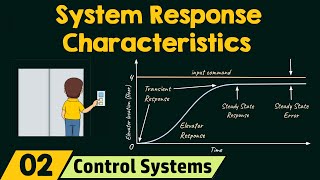
Introduction to Transient Response Examples
🔒 Unlock Audio Lesson
Sign up and enroll to listen to this audio lesson

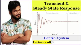
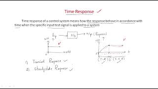
Today, we’re going to dive into some examples of transient responses. Can anyone remind me what we defined as transient response in our previous discussions?

It's how the system behaves immediately after an input change, before it reaches a steady-state.
Exactly! Now, let's consider a second-order system and analyze its transient response. What parameters do we think are crucial for this analysis?

Parameters like rise time, overshoot, and settling time are important.
Correct! These parameters help us understand how quickly our system reacts and stabilizes. We'll explore these in our examples.
Detailed Analysis of a Second-order System
🔒 Unlock Audio Lesson
Sign up and enroll to listen to this audio lesson

Let’s examine a specific transfer function: G(s) = 10 / (s² + 4s + 10). Can someone help me identify the damping ratio and natural frequency from this?

The damping ratio can be found from the coefficients. Here, we find ζ from 2ζω_n = 4, so ζ = 0.2.
Right! And what does this damp ratio imply about our system's transient response?

Since it's less than 1, it indicates the system is underdamped and will oscillate before settling.
Excellent observation! Understanding these parameters allows us to predict system behavior effectively.
Calculating Key Transient Parameters
🔒 Unlock Audio Lesson
Sign up and enroll to listen to this audio lesson
Now, let's say we have identified the damping ratio and natural frequency. Can anyone tell me how we would calculate the rise time?
I think the formula involves the damping ratio and natural frequency, right?
Yes! The rise time for a second-order underdamped system is typically approximated as trt ≈ π / (ω_n √(1 - ζ²)). Let's calculate that together.
So for ζ = 0.2 and ω_n = 5, we can substitute and solve!
Exactly! Make sure to perform these calculations to analyze how quickly the system approaches its desired value.
Implications of Steady-State Responses in Control Systems
🔒 Unlock Audio Lesson
Sign up and enroll to listen to this audio lesson
Let's shift gears to steady-state responses. Why is it important to analyze this after understanding the transient response?
The steady-state tells us how accurate our system is over time, after all fluctuations are settled.
Exactly! We use error constants like Kp, Kv, and Ka to quantify these errors. Why don’t we do an exercise to find steady-state error from the example we discussed?
Sure! If Kp = 10, then the steady-state error for a step input would be ess = 1 / (1 + Kp) = 0.09.
Great job! This ensures we not only understand how our system responds initially, but also how it performs in a stable state.
Introduction & Overview
Read summaries of the section's main ideas at different levels of detail.
Quick Overview
Standard
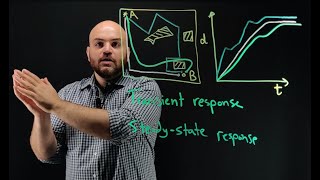
The section elaborates on examples that illustrate transient and steady-state responses of control systems, highlighting the importance of parameters like rise time, overshoot, and settling time.
Detailed
In this section, we examine specific examples of transient and steady-state responses in control systems, illustrating how these responses manifest in various scenarios. It emphasizes the calculations of key parameters like rise time, settling time, and steady-state error, and explores the implications of damping ratio and natural frequency on system behavior. By understanding these examples, students can better grasp the practical applications of theoretical concepts in control systems.
Youtube Videos


Audio Book
Dive deep into the subject with an immersive audiobook experience.
Example of Transient Response Calculation
Chapter 1 of 1
🔒 Unlock Audio Chapter
Sign up and enroll to access the full audio experience
Chapter Content
For a system with ζ=0.5 and ωn=5 rad/s, the rise time and settling time can be calculated, and the transient response will show oscillations that decay over time.
Detailed Explanation
In this example, we are looking at a specific system characterized by a damping ratio of 0.5 and a natural frequency of 5 rad/s. The damping ratio indicates that the system is underdamped, meaning it will demonstrate oscillatory behavior before settling down to its steady-state value. The rise time is the time it takes for the system's response to go from 10% to 90% of its final value, which can be calculated using standard formulas relating to the damping ratio and natural frequency. The settling time similarly reflects how long it takes for the output to remain within a certain percentage of the final value after any disturbances. This example illustrates how the parameters ζ and ωn directly impact the performance of the system and how they can be mathematically analyzed to predict system behavior after a change in input.
Examples & Analogies
Think of a swing in a playground. If you push it gently (the input change), it will swing back and forth a few times (oscillations) before eventually coming to a stop at a position where it settles (steady-state). If you push too hard or too soft, it will take longer to settle down. Similarly, in our system with ζ=0.5, we can imagine that with each push, the swing moves closer to the final resting position, demonstrating how the system responds to changes.
Key Concepts
-
Transient Response: The immediate output behavior post-input change.
-
Damping Ratio (ζ): A measure of how oscillations decay over time in a system.
-
Natural Frequency (ωn): Indicates how fast the system will oscillate when not damped.
-
Overshoot: The peak value of the output exceeding the steady-state value.
-
Settling Time (tst): Time required for the output to settle within a range of its final value.
-
Steady-State Response: System behavior after transient effects have dissipated.
Examples & Applications
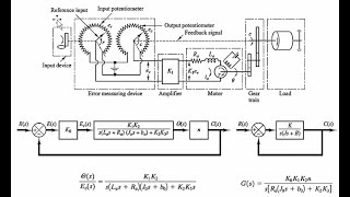
Example of a second-order system: G(s) = 10 / (s² + 4s + 10) to demonstrate damped oscillations.
Calculating rise time and settling time based on given damping ratio and natural frequency.
Memory Aids
Interactive tools to help you remember key concepts
Rhymes
In a damped state, we oscillate, but don’t take too long to settle straight.
Stories
Imagine a boat rocking on a lake. The faster it stabilizes after a wave, the better the damping; too much rocking means slow settling down.
Memory Tools
R.O.S.E. - Rise time, Overshoot, Settling time, Error steady-state for control analysis.
Acronyms
D.O.N.E - Damping, Overshoot, Natural frequency, Error for system performance.
Flash Cards
Glossary
- Transient Response
The output behavior of a system immediately after a change in input.
- Damping Ratio (ζ)
A dimensionless measure describing the amount of damping in a system.
- Natural Frequency (ωn)
The frequency at which a system oscillates in the absence of damping.
- Settling Time (tst)
The time required for the output to remain within a certain range of the final value.
- Overshoot
The maximum peak value of the output beyond the steady-state value.
- SteadyState Response
The behavior of the system after it has reached equilibrium.
Reference links
Supplementary resources to enhance your learning experience.