
Step Input
Enroll to start learning
You’ve not yet enrolled in this course. Please enroll for free to listen to audio lessons, classroom podcasts and take practice test.
Interactive Audio Lesson
Listen to a student-teacher conversation explaining the topic in a relatable way.
Understanding Step Input Response
🔒 Unlock Audio Lesson
Sign up and enroll to listen to this audio lesson

Today, we'll discuss the step input response of control systems. Can anyone tell me what a step input is?

A step input is when the input to the system changes suddenly, like switching on a light.
Correct! It’s a sudden change. Now, how do we analyze a system's response to this change?

We look at the transient and steady-state responses?
Exactly! Let’s start with the transient response. Who can name some key characteristics of it?

There’s rise time, settling time, and overshoot!
Good job! Remember the acronym RSO to help you recall those: Rise time, Settling time, and Overshoot. Now, what do you think overshoot signifies in a system’s response?

It shows how much the output exceeds the final value before settling down.
Exactly! It reflects the system's ability to quickly adapt to changes while maintaining control. Let’s summarize: The transient response is crucial for understanding how quickly and effectively the system stabilizes after a step input.
Factors Affecting Transient Response
🔒 Unlock Audio Lesson
Sign up and enroll to listen to this audio lesson

Now, let's explore the factors affecting the transient response. What role does damping play?
Higher damping means less oscillation, right?
Absolutely! The damping ratio ζ is vital for controlling overshoot and settling time. What happens with an underdamped system?
It oscillates before settling down.
Correct! And how about the natural frequency? What does that tell us?
It indicates how fast the system can respond to changes.
Well done! The natural frequency ωn shows the oscillation speed. Let’s review: Damping influences the oscillation behavior, while natural frequency indicates response speed. Remember, RSO!
Steady-State Response
🔒 Unlock Audio Lesson
Sign up and enroll to listen to this audio lesson
Now shifting to the steady-state response. Why is it important to analyze steady-state error?
It tells us how accurate the system is in the long run.
Exactly! The steady-state error can be evaluated using error constants. Who can tell me about Kp?
Kp is the position error constant for step inputs.
Right! And the formula for steady-state error with Kp is what?
ess = 1 / (1 + Kp).
Great! This indicates how we measure discrepancies between desired and actual output. Let's conclude our discussion by summarizing: steady-state response is essential for performance assessment in control systems.
Introduction & Overview
Read summaries of the section's main ideas at different levels of detail.
Quick Overview
Standard
In this section, the chapter focuses on the step input response of control systems, detailing key aspects like rise time, settling time, overshoot, and how steady-state errors are affected by various error constants.
Detailed
Step Input Response
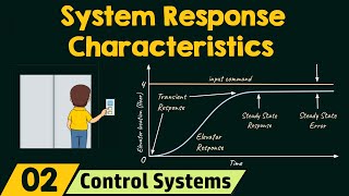
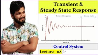
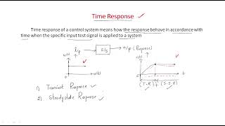
In control systems, the response to a step input is a crucial aspect of assessing system performance. The step input is characterized by the immediate behavior of the system when a constant input is applied. This section explores both the transient and steady-state responses to a step input:
Transient Response
The transient response shows how the output varies from its initial state until it stabilizes after a step input. Important features include:
- Rise Time (trt_r): Time taken for the output to rise from 10% to 90% of its final value.
- Settling Time (tst_s): Time needed for the output to remain within a certain percentage of the final value.
- Overshoot (MpM_p): The maximum amount the output exceeds its final steady-state value.
These factors are influenced by the Damping Ratio (ζ) and Natural Frequency (ωn), which determine the oscillatory behavior of the system.
Steady-State Response
Once the system stabilizes, the steady-state response reveals how the output behaves to prolonged step inputs. It is analyzed using steady-state error and error constants:
- Position Error Constant (Kp): Relates to steady-state error for step inputs, indicating the accuracy of the system.
- Formula: For a step input, the steady-state error is:
ess = 1 / (1 + Kp)
The chapter emphasizes the importance of these aspects for designing effective control systems, highlighting that both the transient and steady-state responses are essential to ensure system performance in terms of speed and accuracy.
Youtube Videos


Audio Book
Dive deep into the subject with an immersive audiobook experience.
Understanding Steady-State Response
Chapter 1 of 6
🔒 Unlock Audio Chapter
Sign up and enroll to access the full audio experience
Chapter Content
Once the system has settled and transient effects have subsided, the system reaches a steady state. The steady-state response describes how the output behaves in response to a constant input after the transient effects die out.
Detailed Explanation
When we talk about a system reaching a 'steady state,' we mean that it has stabilized after any initial disturbances or changes in input. This is typically what happens after the transient responses (initial reactions) have faded away. Once in steady state, the system consistently produces a particular output in response to a constant input, indicating that it is functioning normally and predictably.
Examples & Analogies
Imagine boiling water in a pot. When you first turn on the heat (the input), the water experiences changes: it heats up and bubbles as it starts to boil. However, once it reaches a steady boil (the steady state), the water continues to bubble consistently, reflecting that the system (the pot and water) has adjusted to the constant heat input.
Key Factors in Analyzing Steady-State Response
Chapter 2 of 6
🔒 Unlock Audio Chapter
Sign up and enroll to access the full audio experience
Chapter Content
Key factors in analyzing steady-state response include:
1. Steady-State Error: The difference between the desired output and the actual output as time approaches infinity.
- Types of Inputs: Step input, ramp input, or parabolic input.
- Error Constants: The steady-state error for each type of input can be determined using error constants.
Detailed Explanation
To analyze steady-state response effectively, we need to consider the 'steady-state error.' This is the difference between what we want the system to output and what it actually outputs after everything has settled down. Different types of inputs (like steps, ramps, or parabolic changes) can affect how we calculate this error. We use specific constants (error constants) to quantify how much error occurs under each condition, enabling us to tailor our systems better.
Examples & Analogies
Think about a thermostat in your home set to maintain a specific temperature. If you set it to 70 degrees Fahrenheit, the 'steady-state error' occurs if the actual room temperature stabilizes at, say, 68 degrees instead. The difference (2 degrees in this case) represents the steady-state error, which could stem from either the thermostat's calibration or the heating system's efficiency.
Error Constants Explained
Chapter 3 of 6
🔒 Unlock Audio Chapter
Sign up and enroll to access the full audio experience
Chapter Content
- Error Constants:
- Position Error Constant Kp: Determines the steady-state error for a step input.
- Velocity Error Constant Kv: Determines the steady-state error for a ramp input.
- Acceleration Error Constant Ka: Determines the steady-state error for a parabolic input.
Detailed Explanation
Error constants are specific values that help us predict how much steady-state error will occur for different situations. The Position Error Constant (Kp) is used for step inputs, which jump suddenly and require the system to react to a new constant output. The Velocity Error Constant (Kv) is relevant for ramp inputs, where there’s a gradual increase in input over time. Lastly, the Acceleration Error Constant (Ka) deals with parabolic inputs that involve changes in acceleration. Each of these constants plays a crucial role in calculating and understanding the expected error in responses.
Examples & Analogies
You can think of error constants like different switches for lights in a room. If you flip a switch (a step input), you want the light to come on immediately (Kp). If you slowly dim the lights (a ramp input), you can think of how quickly the lights adjust to this change with Kv. If you’re adding more lights progressively (like accelerating the input), Ka would tell us how well our system manages this increase so that the lights adjust at the right pace.
Steady-State Error for Different Inputs
Chapter 4 of 6
🔒 Unlock Audio Chapter
Sign up and enroll to access the full audio experience
Chapter Content
- Steady-State Error for Different Inputs:
- For a step input, the error depends on Kp.
- For a ramp input, the error depends on Kv.
- For a parabolic input, the error depends on Ka.
Detailed Explanation
The type of input that we apply to the system significantly influences the steady-state error we will observe. For instance, if you introduce a step input, the steady-state error will primarily hinge on the Position Error Constant (Kp). Similarly, with a ramp input, the error relates to the Velocity Error Constant (Kv). Lastly, when applying a parabolic input, it is the Acceleration Error Constant (Ka) that dictates the potential steady-state error. Understanding these relationships helps engineers fine-tune systems for optimal performance.
Examples & Analogies
Envision a delivery service adapting to various delivery orders. If you place a sudden order (step input), the mild delay in fulfilling may impact the service speed (Kp). For a steady stream of orders (ramp input), efficiency in handling ongoing requests becomes pertinent (Kv). With a spike in demand occurring rapidly (parabolic input), the delivery service must effectively manage this change to avoid delays, reflecting how Ka affects performance under stress.
Steady-State Error Formulae
Chapter 5 of 6
🔒 Unlock Audio Chapter
Sign up and enroll to access the full audio experience
Chapter Content
Steady-State Error Formulae:
- Step Input: For a system with a transfer function G(s), the steady-state error for a step input R(s) = 1/s is given by:
ess = 1 / (1 + Kp)
- Ramp Input: The steady-state error for a ramp input R(s) = 1/s^2 is given by:
ess = 1 / Kv
- Parabolic Input: The steady-state error for a parabolic input R(s) = 1/s^3 is given by:
ess = 1 / Ka
Detailed Explanation
The formulas provided serve as concise methods for calculating steady-state error based on the type of input. For a step input, we can use the Position Error Constant (Kp) to find out how close our system output is to what we desired. The error for a ramp input can be obtained through the Velocity Error Constant (Kv), and for higher-order inputs like parabolic, the formula relies on the Acceleration Error Constant (Ka). These equations simplify the process of evaluating system performance and are essential tools in control system design.
Examples & Analogies
Think of these formulas like measurement tools in baking. If you want to make a cake (achieve your desired output), knowing how much flour to add (Kp, Kv, or Ka) helps you achieve the perfect consistency whether you're making a traditional cake, cupcake (step input), or a soufflé (parabolic input). Each formula is your guide in measuring accurately based on the result you want to achieve.
Example of Steady-State Error Calculation
Chapter 6 of 6
🔒 Unlock Audio Chapter
Sign up and enroll to access the full audio experience
Chapter Content
Example: For a system with Kp = 10, the steady-state error for a step input is:
ess = 1 / (1 + 10) = 0.09
Detailed Explanation
This example illustrates how to calculate steady-state error for a system with a known position error constant (Kp). By substituting Kp into the formula, we can determine that the steady-state error, in this case, is 0.09. This means our desired output differs from the actual output by this small amount, and the calculation shows how effective the system will be at meeting its output targets, highlighting the importance of Kp in controlling the error.
Examples & Analogies
Imagine you're following a recipe that calls for 10 ounces of sugar to achieve the perfect sweetness in your cake. If you accidentally add a little less (like 9.1 ounces), our calculation shows you how much sweetness you missed out on (the 0.09 in the example). This is crucial because it helps you gauge the impact of small adjustments in measurements to reach your end goal.
Key Concepts
-
Transient Response: The system's behavior immediately after an input change, characterized by rise time, settling time, and overshoot.
-
Steady-State Response: The long-term behavior of the system after it stabilizes under constant input.
-
Steady-State Error: The discrepancy between desired and actual output as time approaches infinity.
Examples & Applications
For a second-order system with a damping ratio of 0.5 and a natural frequency of 5 rad/s, the system will have an oscillatory response with a specific rise time and settling time.
Using Kp=10, the steady-state error for a step input can be calculated as ess = 0.09, indicating the accuracy of the system.
Memory Aids
Interactive tools to help you remember key concepts
Rhymes
Rise time, settling fine, overshoot's a climbing sign.
Stories
Imagine a sprinter taking off at the sound of a gun. He quickly rises, may overshoot the finish line, but eventually settles to a steady pace.
Memory Tools
Remember 'Keys to RSO': R for Rise time, S for Settling time, O for Overshoot.
Acronyms
Use 'DAN' for Damping, Accuracy (Kp), and Natural frequency!
Flash Cards
Glossary
- Step Input
A sudden change in input to a system, characterized by a quick transition from one value to another.
- Transient Response
The behavior of a system immediately after a change in input before it reaches steady-state.
- Rise Time (trt_r)
The time taken for the output to rise from 10% to 90% of its final value.
- Settling Time (tst_s)
The time required for the output to remain within a certain percentage of its final value.
- Overshoot (MpM_p)
The maximum peak value of the output response, expressed as a percentage of the steady-state value.
- Damping Ratio (ζ)
A dimensionless measure that describes the amount of damping in the system.
- Natural Frequency (ωn)
The frequency at which a system oscillates in the absence of damping.
- SteadyState Response
The behavior of the system after it has stabilized and reached equilibrium.
- SteadyState Error
The difference between the desired output and the actual output as time approaches infinity.
Reference links
Supplementary resources to enhance your learning experience.