
Example System Responses
Enroll to start learning
You’ve not yet enrolled in this course. Please enroll for free to listen to audio lessons, classroom podcasts and take practice test.
Interactive Audio Lesson
Listen to a student-teacher conversation explaining the topic in a relatable way.
Introduction to the Example System
🔒 Unlock Audio Lesson
Sign up and enroll to listen to this audio lesson

Today, we'll analyze a second-order system with the transfer function G(s) = 10 / (s^2 + 4s + 10). Can anyone tell me why understanding both transient and steady-state responses is important?

It's essential for evaluating how well the system performs under different operating conditions.
Great! Correctly evaluating the system helps in designing control systems that are stable and fast. Let's discuss transient responses first. What do you think the transient response tells us?

It shows how quickly the system reacts to changes.
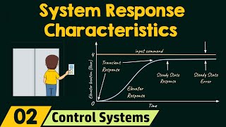
Exactly! Now, transient response can be characterized by parameters like overshoot and settling time. Let’s define each of those.
Transient Response Parameters
🔒 Unlock Audio Lesson
Sign up and enroll to listen to this audio lesson

When we talk about transient response, we often refer to the rise time (trt_r), settling time (tst_s), and overshoot (Mp). Can someone explain what rise time means?

It’s the time it takes for the system output to go from 10% to 90% of the final value.
Absolutely! Now, what about settling time?

That’s the time taken for the output to remain within a certain percentage of the final value.
Perfect! And overshoot, does anyone know what that refers to?
It’s the maximum peak value before the system settles.
Correct! These parameters help us visualize how effective the system is in returning to its desired state after an input change.
Calculating Parameters for the Example System
🔒 Unlock Audio Lesson
Sign up and enroll to listen to this audio lesson
Let's compute the transient parameters for our system. Who can tell me how we can determine the overshoot and settling time using the information from the transfer function?
We can use the damping ratio and the natural frequency related to the transfer function.
Exactly! The transfer function provides the damping ratio and natural frequency needed for these calculations. Can you remind the class what these two factors influence?
They influence the speed and amount of oscillation during transient response.
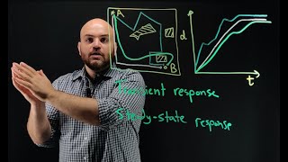
Right! An underdamped system will exhibit oscillations while an overdamped system will return more slowly to steady state. Now, let’s move on to steady-state analysis.
Understanding Steady-State Response
🔒 Unlock Audio Lesson
Sign up and enroll to listen to this audio lesson
What happens once the transient effects have died down?
The system reaches a steady-state where it can maintain a consistent output.
Correct! Now, does anyone recall how we measure steady-state error and what it implies?
The steady-state error is the difference between the desired output and the actual output as time approaches infinity.
Yes! To calculate steady-state error, we often use Kp, the position error constant. What can you tell me about how to determine Kp from the transfer function?
We can calculate Kp by taking the limit of G(s) as s approaches zero.
Well said! Understanding Kp is crucial for ensuring our system performs accurately over time.
Recap and Key Takeaways
🔒 Unlock Audio Lesson
Sign up and enroll to listen to this audio lesson
To wrap up, can anyone summarize why we analyze both transient and steady-state responses in our system?
We need to understand how fast the system responds and how accurately it maintains desired outputs.
And the different damping scenarios can greatly affect the performance during the transient phase!
Excellent points! These analyses are critical for effective design and control in various engineering applications. Always remember, a system's performance relies on both aspects!
Introduction & Overview
Read summaries of the section's main ideas at different levels of detail.
Quick Overview
Standard
In this section, we analyze a second-order system using a given transfer function to demonstrate both transient and steady-state behaviors, focusing on how the system responds to input changes and calculating key parameters like overshoot, settling time, and steady-state error.
Detailed
Detailed Summary
In this section, we explore the transient and steady-state responses of a second-order control system using the transfer function defined as G(s) = 10 / (s^2 + 4s + 10). The focus is on analyzing how this system behaves when subjected to input changes, particularly a step input.
Key Points:
- Transient Analysis: We can derive the system's transient response using Laplace transforms to find critical parameters like overshoot, settling time, and rise time. Understanding these parameters helps evaluate how quickly and effectively the system responds to changes in input.
- Steady-State Analysis: By calculating the steady-state error using the position error constant (Kp), we can understand the system’s performance after the transient effects have subsided. The steady-state analysis is essential for assessing how accurately the system maintains its target response over time.
This section clarifies how both transient and steady-state analyses are interconnected and crucial for effective system design.
Youtube Videos

Audio Book
Dive deep into the subject with an immersive audiobook experience.
Introduction to the Example
Chapter 1 of 3
🔒 Unlock Audio Chapter
Sign up and enroll to access the full audio experience
Chapter Content
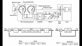
Let's consider an example with a second-order system to better understand both transient and steady-state behaviors. Suppose the system transfer function is:
G(s)=10s2+4s+10G(s) = \frac{10}{s^2 + 4s + 10}
Detailed Explanation
In this example, we are analyzing a second-order system, which is a common type of control system. The system is defined by its transfer function, which represents the relationship between the input and output of the system in the Laplace domain. For our case, the transfer function is G(s) = 10 / (s² + 4s + 10). This function is crucial as it will help us analyze both the transient and steady-state responses of the system after an input change.
Examples & Analogies
Think of the system transfer function like a recipe for baking a cake. Just like a recipe provides the ingredients and steps to follow in order to get the final cake, the transfer function describes how the system behaves based on its parameters.
Transient Analysis
Chapter 2 of 3
🔒 Unlock Audio Chapter
Sign up and enroll to access the full audio experience
Chapter Content
Transient Analysis: By solving for the time-domain response using Laplace transforms, we can obtain the overshoot, settling time, and rise time.
Detailed Explanation
In the transient analysis phase, we focus on how the output of the system reacts immediately after a change in input, which is essential for understanding the behavior of the system during transitions. We use Laplace transforms to convert these time domain responses into a form that allows us to calculate characteristics like overshoot, settling time, and rise time. Overshoot refers to how much the response exceeds its final value during transient conditions, while settling time is how long it takes for the output to stabilize within a certain percentage of the final value. Rise time measures how quickly the system responds to the input change.
Examples & Analogies
Consider an amusement park ride that suddenly starts moving. The time it takes for the ride to go from a standstill to its maximum speed is similar to the rise time. If it overshoots the maximum speed momentarily, that’s like overshoot in our system response. Finally, how long before the ride smooths out and reaches a constant speed corresponds to settling time.
Steady-State Analysis
Chapter 3 of 3
🔒 Unlock Audio Chapter
Sign up and enroll to access the full audio experience
Chapter Content
Steady-State Analysis: If the system is subjected to a step input, the steady-state error can be calculated using KpK_p.
Detailed Explanation
Once the system has passed through the transient phase, we observe its steady-state behavior, which is how the system reacts to a constant input after the transient effects have dissipated. In this case, when the example system receives a step input, we can calculate the steady-state error using the position error constant (Kp). The steady-state error indicates how far the actual output is from the desired output as time progresses towards infinity. This analysis is critical as it helps determine how accurately the system can respond to persistent inputs.
Examples & Analogies
Imagine you are trying to fill a bathtub with water until it reaches a certain level. The water rushing in represents a step input. Initially, as you turn on the faucet, the water level rises quickly (transient response). Once the water reaches the desired level and stabilizes, that’s your steady-state. However, if the water level doesn't exactly match where you want it, there is a steady-state error, which you could fix by adjusting the faucet.
Key Concepts
-
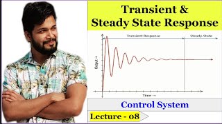
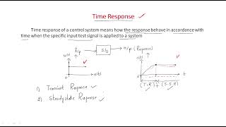
Transient Response: The initial behavior of a system after an input change.
-
Steady-State Response: The system's behavior after transient effects have dissipated.
-
Overshoot: The peak response above the desired system output.
-
Settling Time: The duration for which the output remains within a defined range of the final value.
-
Damping Ratio: Defines how oscillations decay over time in a system.
-
Natural Frequency: The frequency without damping, related to oscillation speed.
-
Steady-State Error: The difference between the desired output and actual output at equilibrium.
-
Position Error Constant (Kp): Measures steady-state error for a step input.
Examples & Applications
Given the transfer function G(s) = 10 / (s^2 + 4s + 10), we calculate that for a certain input, the overshoot is 15%, and settling time is 3 seconds.
Using the calculated Kp = 10, the steady-state error for a step input is found to be ess = 1 / (1 + Kp) = 0.09.
Memory Aids
Interactive tools to help you remember key concepts
Rhymes
When your system starts to sway, overshoot will come to play.
Stories
Imagine a car accelerating to a stop sign—just after it passes the sign, it might roll a bit further—that moment of roll is like overshoot!
Memory Tools
ROSE: Remember Overshoot, Settling Time, and Error response—these are key in transient behavior!
Acronyms
TOSS
Transient Overshoot Settling time Steady state—watch for these in system responses.
Flash Cards
Glossary
- Transient Response
The output behavior of a system immediately after a change in input before it reaches steady-state.
- SteadyState Response
The behavior of the system after it has settled, reflecting its equilibrium condition.
- Overshoot
The maximum peak value of the output response above the steady-state value.
- Settling Time
The time required for the output to remain within a specified percentage of the final value.
- Damping Ratio (ζ)
A dimensionless quantity that indicates how oscillations in a system decay after a disturbance.
- Natural Frequency (ωn)
The frequency at which a system would oscillate if there were no damping.
- SteadyState Error
The difference between the desired output and the actual output as time approaches infinity.
- Position Error Constant (Kp)
Reflects the steady-state error for a step input.
Reference links
Supplementary resources to enhance your learning experience.