
Steady-State Response
Enroll to start learning
You’ve not yet enrolled in this course. Please enroll for free to listen to audio lessons, classroom podcasts and take practice test.
Interactive Audio Lesson
Listen to a student-teacher conversation explaining the topic in a relatable way.
Introduction to Steady-State Response
🔒 Unlock Audio Lesson
Sign up and enroll to listen to this audio lesson

Today, we are going to explore steady-state response. Can anyone tell me what this means?

Is it how the system behaves after all the initial fluctuations?
Exactly! The steady-state response reflects how a system behaves after it has settled. Now, why is it important in control systems?

Because we need to ensure the system is stable and performs accurately.
Correct! This analysis helps us in understanding stability and performance of the system over time.
Steady-State Error and Error Constants
🔒 Unlock Audio Lesson
Sign up and enroll to listen to this audio lesson

Now, let’s discuss steady-state error. What do we understand by this term?

It’s the difference between what we want the output to be and what we actually get over time.
Exactly! And we calculate it using error constants. Can anyone tell me what the Position Error Constant (Kp) does?

Kp tells us the steady-state error for a step input.
Correct! And what about the Velocity Error Constant (Kv) and Acceleration Error Constant (Ka)?
Kv measures error for ramp inputs, and Ka does it for parabolic inputs!
Fantastic! Remembering these constants can greatly help in system design. A mnemonic to remember is 'Kp, Kv, Ka – Step, Ramp, Parabola'!
Types of Input and Steady-State Error Formulae
🔒 Unlock Audio Lesson
Sign up and enroll to listen to this audio lesson
Let’s move on to the types of inputs. Can anyone list them?
I believe there are step, ramp, and parabolic inputs!
Very good! Now, the steady state error can be calculated using specific formulas. What do you think they are?
For step input, it’s ess = 1/(1 + Kp) right?
That's right! And for ramp input it’s ess = 1/Kv, while for parabolic input it’s ess = 1/Ka. Anyone can remember these?
We can remember it like 'ess=1/(1+Kp), ess=1/Kv, ess=1/Ka.'
Exactly! Great teamwork.
Analyzing Steady-State Response
🔒 Unlock Audio Lesson
Sign up and enroll to listen to this audio lesson
Now, let’s apply our knowledge. If we have a system with Kp = 10, what would be the steady-state error for a step input?
We would use the formula ess = 1/(1 + Kp). So, ess = 1/(1 + 10) = 0.09!
Great job! This calculation is crucial for assessing system performance. Can you see how understanding this allows for better design in engineering?
Yes, it helps us improve system accuracy.
Exactly! Remember this as you progress in control systems.
Introduction & Overview
Read summaries of the section's main ideas at different levels of detail.
Quick Overview
Standard
In steady-state response, systems react to constant inputs and display errors relative to the desired output. Its analysis involves understanding various error constants and the steady-state error associated with different types of inputs, such as step, ramp, and parabolic inputs.
Detailed
Steady-State Response
The steady-state response is a critical aspect of control systems that describes how the output behaves once transient effects have diminished, giving us insights into stability and performance over time. In this segment, we focus on key elements of steady-state analysis:
- Steady-State Error: This refers to the discrepancy between the desired and actual output as time approaches infinity. Understanding steady-state error is vital to control system design as it presents reliability metrics when subjected to constant inputs.
- Types of Inputs: The way a system reacts can vary significantly depending on the input type, which can be:
- Step Input
- Ramp Input
-
Parabolic Input
Each input type presents its steady-state characteristics that the designer must understand. - Error Constants: These are parameters that help quantify the steady-state error for various input types:
- Position Error Constant (Kp): Measures the steady-state error for a step input, calculated using the limit of the open-loop transfer function as s approaches zero.
- Velocity Error Constant (Kv): Determines the steady-state error for a ramp input, involving the input multiplied by the transfer function.
- Acceleration Error Constant (Ka): Represents the steady-state error for a parabolic input, related to the second derivative of the input.
- Steady-State Error Formulas:
- For a step input:

- For a ramp input:

- For a parabolic input:

These principles are fundamental for the effective design and evaluation of control systems, ensuring engineers can fulfill speed, accuracy, and consistency benchmarks.
Youtube Videos


Audio Book
Dive deep into the subject with an immersive audiobook experience.
Overview of Steady-State Response
Chapter 1 of 6
🔒 Unlock Audio Chapter
Sign up and enroll to access the full audio experience
Chapter Content
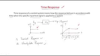
Once the system has settled and transient effects have subsided, the system reaches a steady-state. The steady-state response describes how the output behaves in response to a constant input after the transient effects die out.
Detailed Explanation
The steady-state response is the behavior of a control system after it has had sufficient time to settle down following a change in input. During this phase, the dynamics influenced by transient effects (like overshooting or oscillations) have diminished. The system output stabilizes to a specific value that reflects how the system reacts to constant inputs over time.
Examples & Analogies
Imagine boiling a pot of water. Initially, you will see bubbles and turmoil in the water (transient phase). However, once the water reaches its boiling point and stabilizes, you observe that it stays at that temperature, representing the steady-state response of the system.
Understanding Steady-State Error
Chapter 2 of 6
🔒 Unlock Audio Chapter
Sign up and enroll to access the full audio experience
Chapter Content
- Steady-State Error: The difference between the desired output and the actual output as time approaches infinity.
Detailed Explanation
Steady-state error is a crucial concept that indicates how well a control system can reach its target output when all transient effects have ceased. It is defined as the difference between what the system is supposed to output and what it actually outputs after a long time. Essentially, it tells us how accurate and effective our control system is in tracking its desired value.
Examples & Analogies
Think of a car's cruise control system. If you set it to maintain a speed of 60mph, but the system only manages to hold a speed of 58mph, the steady-state error is 2mph. This error shows how well the cruise control system can maintain the desired speed over time.
Types of Inputs and Their Effects
Chapter 3 of 6
🔒 Unlock Audio Chapter
Sign up and enroll to access the full audio experience
Chapter Content
○ Types of Inputs: Step input, ramp input, or parabolic input.
Detailed Explanation
The type of input provided to a control system significantly affects the system's steady-state response. Common input types include step inputs (a sudden change in input), ramp inputs (a steady increase in input over time), and parabolic inputs (a quadratic increase in input). Each of these inputs influences the steady-state behavior differently, leading to varying degrees of steady-state error.
Examples & Analogies
If you try to feed a plant (the system) a large amount of water all at once (step input), it may overflow and not get absorbed efficiently—leading to a higher steady-state error. Conversely, watering it steadily over time (ramp input), or implementing a very gradual increase in water (parabolic input), allows for better absorption and smaller error.
Error Constants Defined
Chapter 4 of 6
🔒 Unlock Audio Chapter
Sign up and enroll to access the full audio experience
Chapter Content
- Error Constants:
- Position Error Constant Kp: Determines the steady-state error for a step input.
- Velocity Error Constant Kv: Determines the steady-state error for a ramp input.
- Acceleration Error Constant Ka: Determines the steady-state error for a parabolic input.
Detailed Explanation
Error constants are specific values used in control systems to quantify the steady-state error for different types of inputs. The Position Error Constant (Kp) is relevant for step inputs, the Velocity Error Constant (Kv) applies to ramp inputs, and the Acceleration Error Constant (Ka) pertains to parabolic inputs. These constants are crucial for assessing how the system performs across various input scenarios, influencing system design.
Examples & Analogies
Think of Kp, Kv, and Ka as measuring cups for each type of ingredient in a recipe. For a cake (the system) to turn out correctly, having the right amount of flour (Kp for a step input), sugar (Kv for a ramp input), or eggs (Ka for a parabolic input) is crucial. Each ingredient contributes differently to the final taste and texture (steady-state response) of the cake.
Formulating Steady-State Error
Chapter 5 of 6
🔒 Unlock Audio Chapter
Sign up and enroll to access the full audio experience
Chapter Content
Steady-State Error Formulae:
- Step Input: For a system with a transfer function G(s), the steady-state error for a step input R(s)=1/s is given by:
ess=1/(1+Kp)
- Ramp Input: The steady-state error for a ramp input R(s)=1/s^2 is given by:
ess=1/Kv
- Parabolic Input: The steady-state error for a parabolic input R(s)=1/s^3 is given by:
ess=1/Ka
Detailed Explanation
The steady-state error formulae help calculate how far off the actual output is from the desired output for different types of inputs. For a step input, the formula incorporates the Position Error Constant Kp to evaluate how much error to expect once the system settles. Similarly, for ramp and parabolic inputs, the steady-state error depends on Kv and Ka, respectively. These formulae provide engineers with essential tools to evaluate and optimize system performance.
Examples & Analogies
Imagine planning a road trip where you want to end up at a specific destination (desired output). Depending on whether you are driving through flat terrain (step input), up a hill (ramp input), or rounding a bend (parabolic input), your navigation aids (error constants) help you calculate how likely you are to arrive at the right place—and how to adjust your route if needed (steady-state error).
Example Calculation
Chapter 6 of 6
🔒 Unlock Audio Chapter
Sign up and enroll to access the full audio experience
Chapter Content
Example:
For a system with Kp=10, the steady-state error for a step input is:
ess=1/(1+10)=0.09
Detailed Explanation
In this example, the Position Error Constant is given as Kp = 10. By using the formula for steady-state error with a step input, we calculate the steady-state error to be 0.09. This implies that, under given conditions, the system will settle to an output that is 0.09 units away from the desired output value, indicating an efficient performance due to the relatively high value of Kp.
Examples & Analogies
Continuing with the road trip analogy, if your map shows a destination that is 10 miles on the road to your planned route (Kp = 10), a small detour of 0.09 miles can be easily adjusted—showing that your navigation system is quite precise and effective in getting you close to your intended target.
Key Concepts
-
Steady-State Response: Reflects how a system behaves after transient states have faded.
-
Steady-State Error: The error that persists as time approaches infinity.
-
Position Error Constant (Kp): Defines the error for step input.
-
Velocity Error Constant (Kv): Defines the error for ramp input.
-
Acceleration Error Constant (Ka): Defines the error for parabolic input.
Examples & Applications
For a system with Kp = 10, the steady-state error for a step input is ess = 1/(1 + 10) = 0.09.
For a ramp input with Kv = 5, the steady-state error is ess = 1/Kv = 0.2.
Memory Aids
Interactive tools to help you remember key concepts
Rhymes
Kp for steps and Kv for ramps, Ka for parabolic jumps; they define the errors each type clamps.
Stories
Once there was a control system named Steady who wanted to know how well it performed. With friends Kp, Kv, and Ka, each specialized in different inputs, they helped Steady understand how far off it was from its desired goal.
Memory Tools
Remember 'K for Kp, step is first, K for Kv, ramps are for thirst, K for Ka, parabolic is the worst!'
Acronyms
K.E.Y. - K for Kp (step), E for Kv (ramp), Y for Ka (parabola) in steady-state.
Flash Cards
Glossary
- SteadyState Response
The behavior of a system after it has settled and transient effects have diminished.
- SteadyState Error
The difference between the desired output and the actual output as time approaches infinity.
- Position Error Constant (Kp)
A constant that indicates the steady-state error for a step input.
- Velocity Error Constant (Kv)
A constant that indicates the steady-state error for a ramp input.
- Acceleration Error Constant (Ka)
A constant that indicates the steady-state error for a parabolic input.
Reference links
Supplementary resources to enhance your learning experience.