
Parabolic Input
Enroll to start learning
You’ve not yet enrolled in this course. Please enroll for free to listen to audio lessons, classroom podcasts and take practice test.
Interactive Audio Lesson
Listen to a student-teacher conversation explaining the topic in a relatable way.
Understanding Steady-State Error
🔒 Unlock Audio Lesson
Sign up and enroll to listen to this audio lesson

Today, we'll discuss steady-state error, which is crucial for analyzing system performance. Can anyone tell me what steady-state error reflects?

Is it the difference between the desired and actual output as time approaches infinity?
Exactly! So, how do we calculate this error for different types of inputs?

We use specific error constants for each input type.
That's correct, and today, we focus on the parabolic input. Do you remember the formula for steady-state error related to parabolic inputs?

It's derived using the acceleration error constant, Ka?
Exactly! The formula is \( e_{ss} = \frac{1}{K_a} \). Let’s remember that Ka reflects how well our system can follow a parabolic input.
Analyzing Error Constants
🔒 Unlock Audio Lesson
Sign up and enroll to listen to this audio lesson

Can anyone summarize what Ka represents in relation to our system's response?

Ka is the acceleration error constant that indicates the steady-state accuracy of the system for parabolic inputs.
Good! Now, why is it important to analyze the steady-state error for parabolic, ramp, and step inputs?
Because it helps us optimize the control system for different operational scenarios.
That's right! Optimizing control strategies based on input types helps ensure our system remains stable and accurate.
Calculating Steady-State Error for Parabolic Input
🔒 Unlock Audio Lesson
Sign up and enroll to listen to this audio lesson
Let's take a theoretical system where Ka is given as 8. What would be our steady-state error for the parabolic input?
We would use the formula, so \( e_{ss} = \frac{1}{8} = 0.125 \).
Fantastic! This illustrates that the smaller Ka is, the larger the steady-state error becomes. Any reflection on why this occurs?
It’s because a larger Ka means the system can better follow the changing input.
Correct! Tracking accuracy is essential in systems designed for precise control.
Introduction & Overview
Read summaries of the section's main ideas at different levels of detail.
Quick Overview
Standard
In this section, the steady-state response of control systems to parabolic inputs is examined, detailing how to compute the steady-state error using the acceleration error constant. Understanding this behavior is critical for designing effective control systems that can accurately follow parabolic input signals.
Detailed
Steady-State Response to Parabolic Input
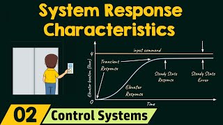
In control systems, the steady-state response characterizes how the output behaves in reaction to sustained inputs, after transient dynamics have passed. This section focuses specifically on parabolic inputs, which represent inputs that change in a quadratic fashion.
Understanding Steady-State Error for Parabolic Inputs
When dealing with parabolic inputs, it's essential to compute the steady-state error, which is a measure of the deviation of the output from the desired value as time progresses towards infinity. The corresponding steady-state error can be calculated using the acceleration error constant, denoted as Ka. The formula for the steady-state error (ess) for a parabolic input is given by:
\[ e_{ss} = \frac{1}{K_a} \]
Error Constants
The acceleration error constant Ka is derived from the system's transfer function and represents how well the system can track changes in parabolic inputs. For higher-order systems, both transient and steady-state responses become increasingly vital for ensuring stability and performance. An understanding of this allows engineers to refine control strategies and optimize system designs to limit steady-state error effectively.
In the broader context of system response analysis, recognizing how the system interacts with various input types, including parabolic, is crucial for creating responsive and accurate control systems. This ensures that any controllable system can operate effectively in real-world applications where inputs are not constant but vary over time in complex ways.
Youtube Videos


Audio Book
Dive deep into the subject with an immersive audiobook experience.
Understanding Steady-State Error
Chapter 1 of 4
🔒 Unlock Audio Chapter
Sign up and enroll to access the full audio experience
Chapter Content
- Steady-State Error: The difference between the desired output and the actual output as time approaches infinity.
Detailed Explanation
Steady-state error describes how well a control system performs when the system output has stabilized after any transients have died down. It is defined as the difference between what we want the output to be (desired output) and what the system actually produces (actual output) when the system has been operating for a long time. This error is critical because it gives us insight into the system's effectiveness in reaching its desired state.
Examples & Analogies
Imagine you are driving a car and you want to reach a specific speed, say 60 mph. After some time of adjusting the accelerator, you eventually settle at 60 mph. However, if the speedometer consistently shows 58 mph instead, the steady-state error here is 2 mph. This shows how well the system (your driving and the car's capability) is performing relative to your goal speed.
Types of Inputs and Error Constants
Chapter 2 of 4
🔒 Unlock Audio Chapter
Sign up and enroll to access the full audio experience
Chapter Content
○ Types of Inputs: Step input, ramp input, or parabolic input.
○ Error Constants: The steady-state error for each type of input can be determined using error constants.
Detailed Explanation
The types of inputs that can be applied to a control system include step inputs (sudden changes), ramp inputs (gradual changes), and parabolic inputs (changes at an accelerating rate). Each type influences the steady-state error in a different way, and specific constants called error constants are used to calculate the steady-state error for these inputs. For instance, for step inputs, we use the position error constant; for ramp inputs, the velocity error constant; and for parabolic inputs, the acceleration error constant.
Examples & Analogies
Think of the differences in driving scenarios: when you make an immediate stop at a red light (step input), when you accelerate steadily on a highway (ramp input), and when you speed up quickly to overtake another vehicle (parabolic input). Each scenario tests the car's ability to respond differently, and just like drivers use different strategies (error constants) to adjust their speed accurately, control systems do the same to minimize errors.
Steady-State Error Formulas
Chapter 3 of 4
🔒 Unlock Audio Chapter
Sign up and enroll to access the full audio experience
Chapter Content
- Steady-State Error for Different Inputs:
○ For a step input, the error depends on KpK_p.
○ For a ramp input, the error depends on KvK_v.
○ For a parabolic input, the error depends on KaK_a.
Detailed Explanation
The steady-state error formula varies depending on the type of input provided to a control system. For example, the steady-state error for a step input is determined using the position error constant (Kp), for a ramp input, it's determined by the velocity error constant (Kv), and for a parabolic input, the acceleration error constant (Ka) is used. These constants reflect the capability of the system to track various input types effectively.
Examples & Analogies
Imagine someone trying to match their walking pace with the pace of a moving escalator (step input), a gently sloped ramp (ramp input), and finally running alongside a moving object at increasing speed (parabolic input). Each activity requires different adjustments based on how quickly the escalator moves (Kp), how long the walk is (Kv), or how rapidly the object accelerates past them (Ka). The effectiveness of their responses is akin to how well a control system minimizes steady-state errors according to input behavior.
Example of Steady-State Error for Parabolic Input
Chapter 4 of 4
🔒 Unlock Audio Chapter
Sign up and enroll to access the full audio experience
Chapter Content
Parabolic Input: The steady-state error for a parabolic input R(s)=1s3R(s) = \frac{1}{s^3} is given by:
\[ e_{ss} = \frac{1}{K_a} \]
Detailed Explanation
When analyzing a parabolic input applied to a control system, we calculate the steady-state error using the formula provided. The output error will be inversely proportional to the acceleration error constant (Ka) of the system. This relationship shows us how well the system compensates for quick changes in input behavior, which tends to be more challenging due to acceleration factors.
Examples & Analogies
Think about trying to catch a ball thrown in a parabolic arc. If you know how fast it accelerates away from you (Ka), you can better anticipate where to position yourself to catch it when it comes down rather than just tracking along a straight path. Just like in control systems, knowing the acceleration allows you to minimize error and catch the ball effectively, reflecting the steady-state adjustment for a parabolic input.
Key Concepts
-
Steady-State Error: A critical measure of performance in control systems, indicating how close the actual output is to the desired output.
-
Acceleration Error Constant (Ka): A key constant that determines how well a system responds to parabolic inputs; lower values indicate a larger steady-state error.
Examples & Applications
If Kp = 10, then the steady-state error for a step input is \( e_{ss} = \frac{1}{1 + K_p} \). For a ramp input, \( Ka = 5 \) yields \( e_{ss} = \frac{1}{5} \). For a parabolic input with Ka = 8, \( e_{ss} = \frac{1}{8} = 0.125 \).
Memory Aids
Interactive tools to help you remember key concepts
Rhymes
Steady-state errors, don’t let them soar, with Ka balanced, you’ll follow much more.
Stories
Imagine a racing car (the system) trying to follow a road that curves gently upwards (the parabolic input). The better its wheels grip the road (the higher the Ka), the closer it stays to the intended path.
Memory Tools
KAP: Ka’s Acceleration Precision – remember that the smaller the Ka, the less precise the tracking.
Acronyms
SSE
Steady-State Error – Remember it as the ultimate measure of your system's end performance after it has settled.
Flash Cards
Glossary
- SteadyState Error
The difference between the desired output and the actual output as time approaches infinity.
- Acceleration Error Constant (Ka)
A term that quantifies a system's ability to follow a parabolic input.
Reference links
Supplementary resources to enhance your learning experience.