
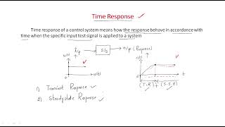
Ramp input
Enroll to start learning
You’ve not yet enrolled in this course. Please enroll for free to listen to audio lessons, classroom podcasts and take practice test.
Interactive Audio Lesson
Listen to a student-teacher conversation explaining the topic in a relatable way.
Understanding Ramp Inputs
🔒 Unlock Audio Lesson
Sign up and enroll to listen to this audio lesson

Today, we’ll explore how control systems respond to ramp inputs. Who can tell me what a ramp input is?

Isn't a ramp input like a steadily increasing or decreasing signal?
Exactly! It represents a constant rate of change. Now, what do you think happens to the steady-state response of a system when it encounters this type of input?

I think the system will take time to stabilize at a new value, but there might be an error involved.
Great observation! This leads us to the idea of steady-state error for different types of inputs.

What is steady-state error exactly?
Good question! Steady-state error is the difference between the desired output and the actual output after the system has settled. For ramp inputs, it's influenced by the velocity error constant, \( K_v \).

So, if we increase the ramp rate, would the error also increase?
Not necessarily. The error's behavior depends on the value of \( K_v \). Remember that formula: \( e_{ss} = \frac{1}{K_v} \).
To summarize, ramp inputs affect the steady-state response significantly, and the steady-state error is essential in understanding this relationship.
Error Constants and Their Importance
🔒 Unlock Audio Lesson
Sign up and enroll to listen to this audio lesson

Now that we have a grasp on ramp inputs, let’s focus on the error constants. Who can name the three important error constants we discussed?
Kp, Kv, and Ka!
Correct! Each constant relates to different types of inputs. Let's dive into \( K_v \) since it’s crucial for ramp inputs. What’s the definition?
It’s the velocity error constant, right?!
Yes! And it helps us calculate the steady-state error for ramp inputs. \( K_v \) is defined as \( \lim_{s \to 0} s \cdot G(s)H(s) \). Why is this limit important?
It shows us how the system behaves as time goes to infinity, right?
Absolutely! It provides insight into how well the system can follow the ramp input without exhibiting significant error.
To conclude, understanding how to evaluate \( K_v \) and calculate \( e_{ss} \) is essential for analyzing system responses to ramp inputs.
Steady-State Error Calculation
🔒 Unlock Audio Lesson
Sign up and enroll to listen to this audio lesson
Let’s apply what we've learned with a quick exercise. If a system has been identified with \( K_v = 20 \), what do you think the steady-state error would be for a ramp input?
I think we would use the formula \( e_{ss} = \frac{1}{K_v} \). So, it should be \( \frac{1}{20} = 0.05 \)!
Exactly! You nailed it! \( 0.05 \) indicates that the system will consistently deviate from the ramp input by this amount in steady state.
What if \( K_v \) were smaller, say \( 5 \)? Would our error increase?
Right again! If you decrease \( K_v \) to \( 5 \), the steady-state error would increase to \( 0.2 \). This demonstrates how important it is to optimize our systems.
To conclude, we’ve used the formula effectively to determine how different values of \( K_v \) impact steady-state error.
Introduction & Overview
Read summaries of the section's main ideas at different levels of detail.
Quick Overview
Standard
In control systems, the steady-state response to ramp inputs is critical for understanding how accurately the system can follow a changing signal over time. This section focuses on identifying and calculating steady-state errors, their dependencies on error constants, and how to interpret steady-state responses for practical applications.
Detailed
Steady-State Response to Ramp Inputs
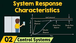
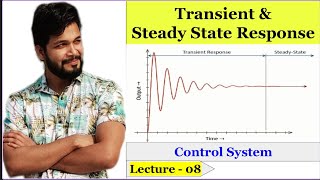
In control systems, understanding how a system responds to different types of inputs is crucial for ensuring accuracy and performance. The steady-state response of a system when subjected to a ramp input is characterized by the steady-state error, which represents the difference between the desired response and the actual output. This section covers:
- Steady-State Error: This error reflects how accurately a system can follow a ramp input as time approaches infinity.
- Error Constants: Specific error constants are vital for determining steady-state errors:
- Position Error Constant ( 4Kp): Measures the error for step inputs.
- Velocity Error Constant (�b4Kv): Determines steady-state errors for ramp inputs, calculated using the formula:
- \( K_v = \lim_{s \to 0} s \cdot G(s)H(s) \)
- Acceleration Error Constant (�b4Ka): Evaluates errors for parabolic inputs, defined as:
- \( K_a = \lim_{s \to 0} s^2 \cdot G(s)H(s) \)
- Steady-State Error Formula for Ramp Input: The formula for steady-state error when subjected to a ramp input (where R(s) = \( \frac{1}{s^2} \)) is:
- \( e_{ss} = \frac{1}{K_v} \)
This section emphasizes the importance of these constants and their formulas in achieving accurate control over systems requiring ramp input responses.
Youtube Videos


Audio Book
Dive deep into the subject with an immersive audiobook experience.
Definition of Steady-State Error for Ramp Input
Chapter 1 of 3
🔒 Unlock Audio Chapter
Sign up and enroll to access the full audio experience
Chapter Content
For a ramp input, the steady-state error depends on the velocity error constant KvK_v.
Detailed Explanation
In control systems, when the input is a ramp, the output doesn't settle instantly, and there will be a steady-state error as the system reacts to this constant increase. The steady-state error is directly related to the system's velocity error constant (Kv), which indicates how well the system can follow the ramp input over time.
Examples & Analogies
Think of a car trying to match the speed of a slowly moving vehicle ahead. If the car can accelerate fast enough (related to Kv), it can keep up with the vehicle's speed increase (the ramp). However, if it can't, there will be a discrepancy (steady-state error) in maintaining the speed.
Steady-State Error Formula for Ramp Input
Chapter 2 of 3
🔒 Unlock Audio Chapter
Sign up and enroll to access the full audio experience
Chapter Content
The steady-state error for a ramp input R(s)=1/s^2R(s) = 1/s^2 is given by: ess=1/Kv e_{ss} = rac{1}{K_v}.
Detailed Explanation
The formula for steady-state error (ess) specifically for a ramp input showcases how it can be quantitatively expressed based on the velocity error constant (Kv). If we know Kv, we can easily compute the steady-state error by taking the reciprocal of Kv. A higher Kv results in a lower steady-state error, indicating better system performance compared to the ramp input.
Examples & Analogies
Consider a heating system trying to maintain a certain temperature while the outside temperature is gradually changing (which can be thought of as a ramp input). If the system's response (Kv) is strong enough, it will closely follow this temperature change. However, if Kv is low, the system will lag behind, resulting in an error in the temperature it finally maintains.
Understanding Error Constants
Chapter 3 of 3
🔒 Unlock Audio Chapter
Sign up and enroll to access the full audio experience
Chapter Content
Error constants help determine the system's steady-state error for different types of inputs, including ramp inputs.
Detailed Explanation
Error constants, such as the position error constant (Kp), velocity error constant (Kv), and acceleration error constant (Ka), are key performance indicators for control systems. For ramp inputs, focus on Kv, which represents how well the system can track changes in the input over time. Each error constant relates to different input types (Kp for step inputs, Kv for ramp inputs, and Ka for parabolic inputs).
Examples & Analogies
Imagine a person learning to ride a skateboard. The more they practice adjusting their balance (velocity), the better they become at following the movements of the skateboard. If they can adjust quickly (high Kv), they will maintain balance even as the skateboard rolls forward (replicating a ramp input). If they are slow to react (low Kv), they may frequently fall off – analogous to a larger steady-state error.
Key Concepts
-
Ramp Input: A type of input signal that represents a constant rate of change over time.
-
Steady-State Error: The difference between the desired and actual output when the system has settled.
-
Velocity Error Constant (Kv): A constant used to calculate steady-state error for ramp inputs, forming part of the control system's feedback.
-
Error Constants: Parameters (Kp, Kv, Ka) that help determine system performance for different input types.
Examples & Applications
For a system with a velocity error constant (Kv) of 15, the steady-state error for a ramp input can be calculated as \( e_{ss} = \frac{1}{15} \approx 0.067 \).
Consider a control system with Kv=0. This means the steady-state error becomes infinite for ramp inputs, indicating the system cannot follow the ramp input accurately.
Memory Aids
Interactive tools to help you remember key concepts
Rhymes
To keep steady and true, Kv must be high, or the error will fly.
Stories
Imagine a race car following a ramp track. If it speeds up slowly, Kv is needed to avoid crashing into inaccuracies in direction!
Memory Tools
Keep Kv high for low error! (K for Kp, V for Kv).
Acronyms
K for Kp, V for Kv, A for Ka - remember the PAS for error constants.
Flash Cards
Glossary
- SteadyState Error
The difference between the desired output and the actual output of a system as time approaches infinity.
- Velocity Error Constant (Kv)
An error constant that measures the steady-state error for a ramp input, defined as \( K_v = \lim_{s \to 0} s \cdot G(s)H(s) \).
- Position Error Constant (Kp)
An error constant that determines the steady-state error for a step input.
- Acceleration Error Constant (Ka)
An error constant that evaluates steady-state error for a parabolic input.
Reference links
Supplementary resources to enhance your learning experience.