
Steady-State Error
Enroll to start learning
You’ve not yet enrolled in this course. Please enroll for free to listen to audio lessons, classroom podcasts and take practice test.
Interactive Audio Lesson
Listen to a student-teacher conversation explaining the topic in a relatable way.
Introduction to Steady-State Error
🔒 Unlock Audio Lesson
Sign up and enroll to listen to this audio lesson

Today we'll discuss steady-state error — the difference between what we want from our control system and what it actually delivers once things settle down.

Why is that important to know?
Excellent question! Knowing the steady-state error helps us evaluate if a system is performing correctly, especially as it reaches stability after changing inputs. Imagine driving a car; if you aim for a speed and it does not reach that speed, that's your error!

So, it's like keeping track of how close we get to our target speed?
Exactly! We want to minimize that difference, so understanding how we calculate it is vital.

Are there different ways this error can show up?
Yes, the error can vary depending on the type of input signal, like step versus ramp inputs.

Can you give an example?
Of course. For a step input, the position error constant Kp comes into play. If Kp is high, we expect lower steady-state error. Let's explore those constants further.
Error Constants Explained
🔒 Unlock Audio Lesson
Sign up and enroll to listen to this audio lesson

Now let’s discuss the error constants starting with Kp, which is crucial for step inputs.
How do we calculate it?
We find Kp by taking the limit of the product of the system's transfer function G(s) and the feedback H(s) as s approaches zero. This constant indicates how well a system can reduce its steady-state error to a step input.
What about for ramp inputs?
Good point! For ramp inputs, we use the velocity error constant Kv. This constant evaluates how well the system handles changes that happen over time.
And is there one for parabolic inputs too?
Yes, we introduce the acceleration error constant Ka for parabolic inputs, which helps assess the system’s response to more complex inputs.
Could you summarize how these constants affect our steady-state error?
Certainly! A higher Kp will mean less error for step inputs, a higher Kv means less error for ramp inputs, and Ka does the same for parabolic inputs. Balancing these constants is key to better accuracy!
Calculating Steady-State Error
🔒 Unlock Audio Lesson
Sign up and enroll to listen to this audio lesson
Let's calculate the steady-state error using the formulas we've discussed.
Okay, what's the formula for a step input again?
For a step input, it’s e_ss = 1 / (1 + Kp). If we know Kp, we can quickly find our steady-state error.
Can I try an example?
Sure! Let’s say Kp is 10. What’s e_ss?
That means e_ss = 1 / (1 + 10) = 1/11 = 0.09!
What if Kp was zero?
Great question! If Kp is zero, we would have an infinite steady-state error for a step input, indicating a poor system performance. It emphasizes the importance of tuning to get better values!
Different Input Types
🔒 Unlock Audio Lesson
Sign up and enroll to listen to this audio lesson
Now, let's look at how steady-state error varies with input types. Earlier we discussed step inputs.
What about ramp inputs?
For ramp inputs, as I mentioned, we use Kv. The formula becomes e_ss = 1 / Kv. This shows how well our system can deal with constantly changing inputs.
And parabolic inputs too?
Exactly! For parabolic inputs, our formula is e_ss = 1 / Ka. Each constant illustrates a system's performance and helps us adjust it for better output.
So, is the goal always to reduce e_ss?
Absolutely! The less steady-state error we have, the more accurately our system meets targets across different input scenarios.
Summary and Application
🔒 Unlock Audio Lesson
Sign up and enroll to listen to this audio lesson
To wrap things up, let’s summarize what we've learned about steady-state error.
We discussed steady-state error formulas for various inputs!
Correct! We also learned about the error constants Kp, Kv, and Ka, their importance, and how they impact our calculations.
How do we use this in real life?
Great question! Engineers use these in designing control systems for everything from cruise control in cars to robotics. Understanding steady-state error ensures optimal performance over time.
So it's about making the system reliable and accurate?
Exactly! A well-tuned system minimizes steady-state error and provides better control and results. Remember, practice adjusting these constants for real systems!
Introduction & Overview
Read summaries of the section's main ideas at different levels of detail.
Quick Overview
Standard
The section on steady-state error discusses the differences between the desired and actual outputs in control systems when responding to constant inputs. It highlights the importance of error constants for different input types—step, ramp, and parabolic—and presents formulas for calculating steady-state error based on these constants.
Detailed
Steady-State Error
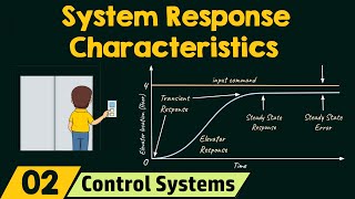
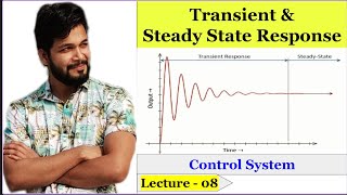
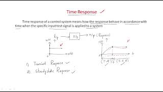
In control systems, after the transient response subsides, the system reaches its steady-state, characterized by its behavior in response to constant inputs. The main focus of this section is on the steady-state error (ess), which represents the discrepancy between the actual output and the desired output as time approaches infinity. This error is crucial for evaluating control system effectiveness and accuracy.
Key Elements of Steady-State Error:
- Types of Inputs: Steady-state error can differ based on the type of input signal—step, ramp, or parabolic.
- Error Constants: Error constants are utilized to determine steady-state errors for various input types:
- Position Error Constant (Kp): Relevant for step inputs, calculated as:
$$ K_p = ext{lim } (s
ightarrow 0) G(s)H(s) $$ - Velocity Error Constant (Kv): Used for ramp inputs, defined as:
$$ K_v = ext{lim } (s
ightarrow 0) s imes G(s)H(s) $$ - Acceleration Error Constant (Ka): Appropriated for parabolic inputs, represented by:
$$ K_a = ext{lim } (s
ightarrow 0) s^2 imes G(s)H(s) $$ - Formulas for Steady-State Error:
- For a step input:
$$ e_{ss} = rac{1}{1 + K_p} $$ - For a ramp input:
$$ e_{ss} = rac{1}{K_v} $$ - For a parabolic input:
$$ e_{ss} = rac{1}{K_a} $$
The importance of these equations lies in their ability to provide insights into how well the control system will perform under different operating conditions, placing emphasis on tuning the error constants for desired steady-state performance.
Youtube Videos


Audio Book
Dive deep into the subject with an immersive audiobook experience.
Definition of Steady-State Error
Chapter 1 of 6
🔒 Unlock Audio Chapter
Sign up and enroll to access the full audio experience
Chapter Content
Once the system has settled and transient effects have subsided, the system reaches a steady-state. The steady-state response describes how the output behaves in response to a constant input after the transient effects die out.
Detailed Explanation
Steady-state error refers to the difference between the output that a control system produces and the output that is required or expected, after the system has had enough time to stabilize. In practical terms, after any initial fluctuations or oscillations have settled down, steady-state error quantifies the system's accuracy in maintaining its desired output during stable operation.
Examples & Analogies
Imagine you're driving a car towards a stop sign. Initially, you may have to brake sharply, causing the vehicle to jerk forward. After a moment, as you glide to a stop, the car finally settles at the stop sign. The position of the stop sign represents your desired output, while where you actually stop, especially if you overshoot or undershoot, represents the steady-state error.
Types of Inputs Affecting Steady-State Error
Chapter 2 of 6
🔒 Unlock Audio Chapter
Sign up and enroll to access the full audio experience
Chapter Content
Key factors in analyzing steady-state response include: 1. Steady-State Error: The difference between the desired output and the actual output as time approaches infinity. - Types of Inputs: Step input, ramp input, or parabolic input.
Detailed Explanation
The steady-state error can be influenced by the type of input the system is receiving, whether it's a step (sudden change), ramp (gradually increasing), or parabolic input (accelerating change). Each of these inputs will challenge the system differently, affecting how accurately the system can reach and maintain the desired output after transient effects have settled.
Examples & Analogies
Consider a home heating system. If you set the thermostat to a specific temperature (step input), the heater needs to reach that temperature quickly. If you gradually increase the desired temperature over time (ramp input), the system has to adjust its heating rate steadily. For a parabolic input, imagine a situation where your desired temperature starts increasing slowly but then accelerates quickly. Each type of input affects how closely the heating system can maintain the set temperature without any long-term deviations.
Error Constants
Chapter 3 of 6
🔒 Unlock Audio Chapter
Sign up and enroll to access the full audio experience
Chapter Content
- Error Constants: - Position Error Constant KpK_p: Determines the steady-state error for a step input. Kp=lim s→0 G(s) H(s) K_p = lim_{s o 0} G(s) H(s) - Velocity Error Constant KvK_v: Determines the steady-state error for a ramp input. Kv=lim s→0 s ⋅ G(s) H(s) K_v = lim_{s o 0} s imes G(s) H(s) - Acceleration Error Constant KaK_a: Determines the steady-state error for a parabolic input. Ka=lim s→0 s^2 ⋅ G(s) H(s) K_a = lim_{s o 0} s^2 imes G(s) H(s)
Detailed Explanation
Error constants are critical for determining how well a system can respond to specific input types. The Position Error Constant (Kp) helps gauge how well the system handles constant inputs, while the Velocity Error Constant (Kv) measures the system's efficiency in responding to gradual inputs, and the Acceleration Error Constant (Ka) assesses for rapidly changing outputs. These constants are derived from the system's transfer function and provide insights into potential steady-state errors.
Examples & Analogies
Think of a teacher grading assignments. If students constantly make the same mistakes (step input), the teacher identifies and addresses them. If students gradually improve their understanding (ramp input), the teacher adjusts the teaching pace accordingly. In the case of students rapidly accelerating their understanding (parabolic input), the teacher must adapt quickly to keep the class on track. The effectiveness of the teacher's responses can be likened to Kp, Kv, and Ka, which determine how accurately the teaching meets students' evolving educational needs.
Steady-State Error for Different Inputs
Chapter 4 of 6
🔒 Unlock Audio Chapter
Sign up and enroll to access the full audio experience
Chapter Content
- Steady-State Error for Different Inputs: - For a step input, the error depends on KpK_p. - For a ramp input, the error depends on KvK_v. - For a parabolic input, the error depends on KaK_a.
Detailed Explanation
The steady-state error for varying types of inputs indicates how responsive the control system is. For example, a system's ability to reach the desired steady state with minimal error for different inputs is reliant on its respective error constant. For a step input, performance primarily hinges on Kp; with a ramp input, it relies on Kv; and for a parabolic input, it is associated with Ka. Understanding this relationship is key to designing systems that can accurately follow diverse input types without substantial deviations.
Examples & Analogies
Imagine you're trying to sail a boat. If the wind suddenly changes direction (step input), you adjust your sails according to the immediate change (Kp). If the wind is gradually increasing in strength (ramp input), you make gradual adjustments to maintain speed and direction (Kv). However, if the wind unexpectedly picks up and becomes gusty (parabolic input), you need to recalibrate quickly to avoid capsizing (Ka). How well you adapt in these scenarios reflects the system’s steady-state error for each input type.
Steady-State Error Formulae
Chapter 5 of 6
🔒 Unlock Audio Chapter
Sign up and enroll to access the full audio experience
Chapter Content
Steady-State Error Formulae: - Step Input: For a system with a transfer function G(s), the steady-state error for a step input R(s)=1/s is given by: ess=1/(1+Kp) e_{ss} = rac{1}{1 + K_p} - Ramp Input: The steady-state error for a ramp input R(s)=1/s^2 is given by: ess=1/Kv e_{ss} = rac{1}{K_v} - Parabolic Input: The steady-state error for a parabolic input R(s)=1/s^3 is given by: ess=1/Ka e_{ss} = rac{1}{K_a}
Detailed Explanation
These formulae provide a numerical way to calculate steady-state error for different input types based on the respective error constants. For each type of input, you can substitute the constant into the formula to find out how much deviation there will be from the desired output once the system reaches stability. This allows designers to predict and minimize errors in system performance.
Examples & Analogies
To put this into context, consider using a calculator to figure out how much gasoline to add to your car based on its current fuel level (step input), your driving habits (ramp input), or the road conditions you anticipate (parabolic input). Using the correct equations helps you determine how much extra gas you might need to maintain optimal performance—just like these formulae help predict steady-state error in control systems.
Example of Steady-State Error Calculation
Chapter 6 of 6
🔒 Unlock Audio Chapter
Sign up and enroll to access the full audio experience
Chapter Content
Example: For a system with Kp=10 K_p = 10, the steady-state error for a step input is: ess=1/(1+10)=0.09 e_{ss} = rac{1}{1 + 10} = 0.09
Detailed Explanation
In this example, if the Position Error Constant (Kp) is 10, the steady-state error when subject to a step input can be calculated using the formula provided. The calculation shows that the system will maintain an error of 0.09 from the desired output. This illustrates how effective the system is at reaching its stable state with minimal deviation.
Examples & Analogies
Think of a barber trying to achieve your desired haircut. If the initial haircut (step input) didn't match your request and the barber keeps adjusting until he gets it as close as possible (using Kp), you could say the difference left over after the final adjustment reflects the steady-state error. In this case, a smaller number like 0.09 indicates he did a great job matching your expectations!
Key Concepts
-
Steady-State Error: Difference between desired and actual output in steady-state.
-
Position Error Constant (Kp): Constant for steady-state error with step input.
-
Velocity Error Constant (Kv): Constant for steady-state error with ramp input.
-
Acceleration Error Constant (Ka): Constant for steady-state error with parabolic input.
Examples & Applications
For a step input with Kp = 10, the steady-state error is calculated as e_ss = 1 / (1 + 10) = 0.09.
For a ramp input with Kv = 5, the steady-state error would be e_ss = 1 / 5 = 0.2.
Memory Aids
Interactive tools to help you remember key concepts
Rhymes
Kp, Kv, and Ka, help our errors to sway, adjusting inputs keep them in play!
Stories
Imagine a race where cars are trying to match a speed limit, Kp helps those cars reach the limit quickly, Kv keeps them there during turns, and Ka ensures they can speed up smoothly at the start.
Memory Tools
Kp = Keep it steady (for steps), Kv = Very fast changes (for ramps), Ka = Accelerate slowly (for parabolas).
Acronyms
E = E – Output difference, Key to performance improvement.
Flash Cards
Glossary
- SteadyState Error
The difference between the desired output and the actual output of a control system as time approaches infinity.
- Position Error Constant (Kp)
A constant that determines the steady-state error for a step input.
- Velocity Error Constant (Kv)
A constant that determines the steady-state error for a ramp input.
- Acceleration Error Constant (Ka)
A constant that determines the steady-state error for a parabolic input.
Reference links
Supplementary resources to enhance your learning experience.