30. Eigenvectors

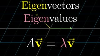
Eigenvectors are fundamental in the study of linear transformations and systems of linear equations. In civil engineering, they are widely used in structural analysis, vibration analysis, stability studies, and finite element methods. Understanding eigenvectors and the corresponding eigenvalues helps civil engineers model physical phenomena such as resonance, stress distribution, and buckling of columns.

Eigenvectors are important concepts in linear algebra, particularly when dealing with matrices. They allow engineers to analyze and predict how structures will react under various forces. In civil engineering, eigenvectors can help determine how structures vibrate and distribute stresses. For example, when a building sways during an earthquake, eigenvectors help calculate how the building's materials will respond to the shaking, ensuring that the structure remains stable and safe.

Think of a swing at a playground. When you push it, it swings back and forth, and this motion has a specific rhythm or pattern. In a similar way, buildings have 'natural' ways of moving when forces are applied to them, and eigenvectors help identify those movements, much like understanding the rhythm of the swing helps you know how far to push it without going too high.

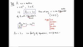
An eigenvector x≠0 of matrix A is a non-zero vector that, when multiplied by the matrix A, yields a scalar multiple of itself: Ax=λx. Here, • x is the eigenvector, • λ∈R (or C) is the eigenvalue associated with x, • A is a square matrix.

An eigenvector is a special type of vector that, when acted upon by a square matrix A, does not change its direction; it only gets scaled (stretched or compressed). The scalar by which it is scaled is known as the eigenvalue (λ). Mathematically, this relationship can be expressed as Ax = λx. In this equation, A transforms the eigenvector x into another vector, but this new vector points in the same direction as the original one, just altered in length.

Imagine you have a rubber band (the eigenvector) that you pull (the matrix A). When you stretch the rubber band, it becomes longer (scaled), but it remains in the same direction no matter how much you pull. The amount by which you stretch it is similar to the eigenvalue. If you pull the rubber band lightly, it extends a little (small eigenvalue). If you pull it hard, it extends a lot (large eigenvalue).

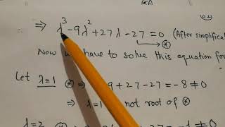
To find eigenvectors, we start by solving the characteristic equation: Ax=λx⇒(A−λI)x=0. This is a homogeneous system of equations, and for a non-trivial solution to exist (i.e., x≠0), the coefficient matrix must be singular: det(A−λI)=0.

The eigenvalue problem involves finding both eigenvalues and eigenvectors of a matrix A. We solve for these by first transforming the equation into a characteristic form, (A − λI)x = 0, where I is the identity matrix. This transformation allows us to find values for λ that tell us what the eigenvalues are. To determine the eigenvalues of the matrix, we compute the determinant of (A − λI) and set it equal to zero. The solutions (roots) of this equation are the eigenvalues, which further allow us to find the corresponding eigenvectors.

Imagine you are tuning a musical instrument, like a guitar. Each string can vibrate at certain frequencies (eigenvalues), and those frequencies correspond to specific notes. The way a string vibrates along its length is akin to its eigenvector. To find out which notes (eigenvalues) your guitar strings can produce, you may pluck the strings and observe their vibrations, just as we solve the characteristic equation to find eigenvalues.

Once the eigenvalues λ are found, each corresponding eigenvector x can be obtained by solving: (A−λI)x=0. This typically results in a system of linear equations, which can be solved using Gaussian elimination or row-reduction.

After calculating eigenvalues, the next step is to find eigenvectors for each eigenvalue. This involves substituting each eigenvalue into the equation (A − λI)x = 0. The result is a linear system of equations which can be resolved using techniques like Gaussian elimination or row-reduction, resulting in the eigenvectors that correspond to each eigenvalue. Each eigenvector indicates a direction in which the matrix transformation only scales the vector without altering its direction.

Think of this process like fitting different puzzle pieces (eigenvectors) into a puzzle board (the matrix). Each piece fits perfectly in a specific orientation that highlights its unique shape (its eigenvalue). Once you know a piece's orientation based on its characteristics (its eigenvalue), you can find how it fits in the larger puzzle, allowing you to see the bigger picture of how everything connects.

1. Linearly Independent Eigenvectors: If matrix A has n distinct eigenvalues, the corresponding eigenvectors are linearly independent.
2. Scaling: Eigenvectors are not unique. If x is an eigenvector, so is kx for any non-zero scalar k.
3. Diagonalization: If A has n linearly independent eigenvectors, then it is diagonalizable: A=PDP⁻¹.
4. Symmetric Matrices: All eigenvalues of a real symmetric matrix are real, and eigenvectors corresponding to distinct eigenvalues are orthogonal.

Eigenvectors have several important properties that are useful in various applications. Firstly, if a matrix has 'n' different eigenvalues, then it will also have 'n' linearly independent eigenvectors, which provide a basis for the vector space. Secondly, although eigenvectors provide unique directions, they can be scaled, meaning that any non-zero multiple of an eigenvector is also an eigenvector. Furthermore, if a matrix has enough eigenvectors, it can be simplified into a diagonal form, which makes computations easier. For symmetric matrices, the eigenvalues are guaranteed to be real, and eigenvectors for different eigenvalues are orthogonal, which further aids in analysis.

Consider a colorful kite flying in the wind. Each color represents a unique eigenvector that captures the kite's behavior in the wind (its direction). However, you can blow the kite harder or softer, thus changing its size while maintaining its shape (scaling). If you had multiple colorful kites, each representing a unique trajectory, together they would show you the entire beautiful array of how the kites navigate the air currents (the matrix's behavior).

An eigenvector represents a direction in which a linear transformation acts as a simple scaling, and the corresponding eigenvalue represents the scale factor. • If λ>1: Stretching • If 0<λ<1: Compression • If λ=−1: Reversal of direction • If λ=0: Maps to zero vector.

Geometrically, eigenvectors can be seen as directions along which the transformation represented by the matrix acts as a simple scaling operation. The eigenvalue associated with an eigenvector indicates the type of scaling behavior. If the eigenvalue is greater than one (λ>1), the vector is stretched; if it is between zero and one (0<λ<1), the vector is compressed; if equal to -1 (λ=-1), the vector reverses direction; and if equal to zero (λ=0), the vector collapses to the zero vector.

Imagine a rubber band that you stretch. If you pull it until it's twice as long (λ>1), you're stretching it; if you gently pinch it to about half its size (0<λ<1), it compresses. Reversing direction is like flipping the band so it snaps back the other way (λ=-1), and ultimately, if you cut the rubber band, it no longer exists (λ=0). Each of these changes represents a unique behavior similar to eigenvalues affecting eigenvectors during transformations.

--