
Fourier Transform vs Laplace Transform in PDEs
Enroll to start learning
You’ve not yet enrolled in this course. Please enroll for free to listen to audio lessons, classroom podcasts and take practice test.
Interactive Audio Lesson
Listen to a student-teacher conversation explaining the topic in a relatable way.
Using Fourier Transform for PDEs
🔒 Unlock Audio Lesson
Sign up and enroll to listen to this audio lesson

Today we'll begin by exploring how Fourier transforms are applied in partial differential equations. Can anyone tell me when we usually use Fourier transforms?

Are they used for infinite or periodic domains?
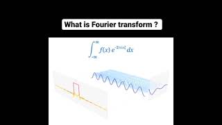
Exactly! Fourier transforms are particularly useful in analyzing problems over infinite or periodic domains. For instance, consider the heat equation defined on an infinite line: ∂u/∂t = α ∂²u/∂x². The Fourier transform helps us handle such scenarios effectively.

So, how does applying the Fourier transform change the equation?
Great question! When we apply the Fourier transform, we convert the spatial variable into a frequency variable, which allows us to solve the time part as an ODE. This simplifies the process considerably.

What do we do after we find the solution?
After obtaining the solution in the frequency domain, we apply the inverse Fourier transform to revert back to the time domain. Keep this process in mind—it’s a fundamental technique!

This sounds a lot like the methods we learned in earlier chapters about signal processing!
Exactly, the connection is crucial! Understanding Fourier transforms' role in PDEs enhances our problem-solving toolkit.
In summary, recall that we use Fourier transforms for infinite or periodic domains to analyze the spatial aspects of PDEs.
Application of Laplace Transform in PDEs
🔒 Unlock Audio Lesson
Sign up and enroll to listen to this audio lesson

Now, let's switch gears and discuss Laplace transforms. Who can remind me when it's best to use Laplace transforms?
They’re used for semi-infinite domains, right?
Exactly! Laplace transforms are particularly effective for problems defined for t ≥ 0. They also handle initial conditions adeptly, which is essential in many engineering applications.
Could you show us an example?
Certainly! Let’s look at the same heat equation you encountered with the Fourier transform, but now we apply the Laplace transform. This approach deals directly with the time variable, making it easier to manage initial conditions.
What happens after that?
After transforming, you will solve the resulting spatial ODE, and then apply the inverse Laplace transform to find the solution in the time domain. This method provides insights for transient analysis.
So creating a solution involves transforming, solving, and inverting—got it!
Precisely! It’s a systematic process indispensable in many civil engineering applications. To recap: Laplace transforms handle semi-infinite domains and are your go-to method for initial conditions and transient behavior.
Comparing the Two Transforms
🔒 Unlock Audio Lesson
Sign up and enroll to listen to this audio lesson
Having explored both transforms, how would you summarize the differences? What contexts do they suit best?
Fourier transforms are for infinite domains or periodic problems, whereas Laplace transforms are for semi-infinite domains.
That’s spot on! Additionally, remember that Fourier transforms focus on frequency analysis, while Laplace transforms involve time-domain analysis.
Does that mean Laplace transforms are better for problems with discontinuities?
Yes! Laplace transforms adeptly manage piecewise functions and discontinuities, making them versatile in civil engineering applications.
So they both have their strengths depending on the type of problem?
Exactly! They complement each other in solving complex engineering problems. To summarize, use Fourier transforms for infinite or periodic domains, and Laplace transforms for handling semi-infinite domains and initial conditions.
Introduction & Overview
Read summaries of the section's main ideas at different levels of detail.
Quick Overview
Standard
The section outlines the appropriate contexts for using Fourier and Laplace transforms in solving PDEs. It explains that Fourier transforms are suited for infinite or periodic domains, while Laplace transforms excel in semi-infinite domains, especially with initial conditions, as exemplified by their use in the heat equation.
Detailed
In this section, we analyze the distinct contexts in which Fourier and Laplace transforms are utilized in the realm of partial differential equations (PDEs). The Fourier transform is ideal for problems defined on infinite or periodic domains, as it allows for the spatial analysis of signals or structures. For instance, applying the Fourier transform to the heat equation results in an ordinary differential equation (ODE) in time. Conversely, Laplace transforms are employed in scenarios involving semi-infinite domains or where initial conditions are critical. This is particularly illustrated by applying the Laplace transform to the same heat equation, which transforms the problem into a more manageable form for analysis. Understanding these distinctions aids civil engineers in selecting the appropriate mathematical tools for specific engineering problems.
Youtube Videos


Audio Book
Dive deep into the subject with an immersive audiobook experience.
Fourier Transform in PDEs
Chapter 1 of 2
🔒 Unlock Audio Chapter
Sign up and enroll to access the full audio experience
Chapter Content
Used in problems with:
- Infinite or periodic domains
- Spatial analysis of signals or structures
Example: Heat equation ∂u = α∂²u on −∞
Detailed Explanation
The Fourier Transform is particularly effective in solving partial differential equations (PDEs) that involve infinite or periodic domains. This means it can easily handle problems that are not confined to a limited area, such as understanding how heat spreads over an entire space. In the heat equation example given, we're looking at how heat changes over time and space.
To solve this, we first apply the Fourier Transform along the x-axis (the spatial dimension), which turns the PDE into an ordinary differential equation (ODE) in time (t). Solving this ODE generally is more straightforward. After finding the solution in the frequency domain, we use the inverse Fourier Transform to revert back to the original spatial and temporal context. This two-step process is powerful because it simplifies complex problems into manageable algebraic equations.
Examples & Analogies
Imagine you are trying to understand how the temperature in a long metal rod changes over time when one end is heated. Instead of analyzing the entire rod at once, you could first look at the heat distribution as if it were a wave moving through the rod — this is similar to using the Fourier Transform. Just as sound waves can be broken down into different frequencies, the heat distribution can be analyzed in terms of its 'frequency' of change. Once you understand the frequency changes, you can figure out the actual temperature distribution at any point in time along the rod.
Laplace Transform in PDEs
Chapter 2 of 2
🔒 Unlock Audio Chapter
Sign up and enroll to access the full audio experience
Chapter Content
Used in problems with:
- Semi-infinite domains
- Initial conditions or transient analysis
Example: Same heat equation on x ≥ 0, apply Laplace transform in t, solve spatial ODE in x, then invert.
Detailed Explanation
The Laplace Transform is ideally suited for solving PDEs that have semi-infinite domains or initial conditions. This makes it particularly useful when dealing with problems like the heat equation that starts at a specific point in time but is only defined for values of x greater than or equal to zero.
In our example, we apply the Laplace Transform in the time domain (t), which simplifies the way we deal with time-dependent changes. This transforms the PDE into an ODE in the spatial variable (x), which we then solve. After finding the solution in the s-domain (the domain of the Laplace Transform), we again apply the inverse Laplace Transform to revert back to a function that describes how heat changes over time and space. This method allows us to track how the heat evolves from an initial state, shedding light on processes like transient heat conduction effectively.
Examples & Analogies
Consider a water tank heating scenario where we want to analyze how the water temperature changes after we turn on the heater at a specific time. We might not be interested in what happens before the heater turns on, making our domain semi-infinite because it only counts from that moment onward. By using the Laplace Transform, we convert the problem of waiting for the water temperature to reach a certain value into a simpler algebraic equation. Solving this will help us understand the heating process and predict the temperature over time, just like figuring out how a plant grows after you water it from a specific point onward.
Key Concepts
-
Fourier Transform: Useful for infinite or periodic domains in PDEs.
-
Laplace Transform: Ideal for semi-infinite domains and managing initial conditions in PDEs.
-
PDEs: Essential equations modeling phenomena in engineering and science.
Examples & Applications
Applying Fourier transform on the heat equation on -∞ < x < ∞ to transform it into an ODE in time.
Applying Laplace transform on the same heat equation on x ≥ 0 to focus on initial value problems.
Memory Aids
Interactive tools to help you remember key concepts
Rhymes
Fourier transforms glow like the moon, turning functions' lights to frequency tunes.
Memory Tools
FLIP - Fourier for Long Infinite Periods, Laplace for Initial Problems.
Acronyms
FITS - Fourier in Time Series, Laplace In Initial States.
Flash Cards
Glossary
- Fourier Transform
A mathematical operation that transforms a function of time into a function of frequency, mainly used for periodic or infinite problems.
- Laplace Transform
A mathematical operation that transforms a function defined for t ≥ 0 into a function of a complex variable, useful for solving differential equations with initial conditions.
- Partial Differential Equations (PDEs)
Equations that involve functions of several variables and their partial derivatives, used extensively in engineering for modeling physical phenomena.
Reference links
Supplementary resources to enhance your learning experience.