
Laplace Transform of Standard Functions
Enroll to start learning
You’ve not yet enrolled in this course. Please enroll for free to listen to audio lessons, classroom podcasts and take practice test.
Interactive Audio Lesson
Listen to a student-teacher conversation explaining the topic in a relatable way.
Introduction to Laplace Transforms
🔒 Unlock Audio Lesson
Sign up and enroll to listen to this audio lesson

Today we're going to discuss the Laplace transform of standard functions. Can anyone tell me why Laplace transforms are important in engineering?

Are they used to simplify differential equations?
Exactly! They convert differential equations into algebraic equations, which are much easier to solve. Let's start with the simplest form, the Laplace transform of a constant function f(t) = 1.

What is the transform for that?
Good question! For f(t) = 1, the Laplace transform is F(s) = 1/s. Remember, this is true as long as s > 0, indicating the region of convergence. Think of 's' as a control parameter!
Laplace Transform of Polynomial Functions
🔒 Unlock Audio Lesson
Sign up and enroll to listen to this audio lesson

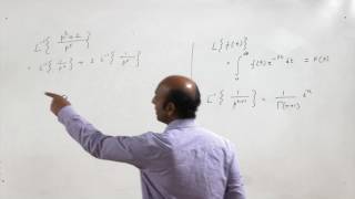
Now, let's talk about polynomial functions. If we have a function f(t) = t^n, what do you think happens with its Laplace transform?

Is it something like F(s) = n!/s^(n+1)?
Correct! F(s) = n!/s^(n+1) utilizes the factorial of n. This relationship helps us handle differential equations involving polynomial terms effectively.

So if n is 2, the transform would be 2!/s^3 which is 2/s^3?
Yes! That's right. Keep in mind how these transforms allow us to manage higher-order polynomials with ease!
Exponentials and Their Transforms
🔒 Unlock Audio Lesson
Sign up and enroll to listen to this audio lesson
Next, let's discuss exponential functions. If our function is f(t) = e^(at), who can tell me the corresponding Laplace transform?
I think it’s F(s) = 1/(s-a)!
Does that mean it only works if s is greater than a?
Exactly! That’s a crucial point. This ensures convergence to the transform we're using. Exponentials are quite common in engineering applications for modeling growth and decay.
Sine and Cosine Transforms
🔒 Unlock Audio Lesson
Sign up and enroll to listen to this audio lesson
Let’s move on to trigonometric functions. We have f(t) = sin(at) and f(t) = cos(at). What are their Laplace transforms?
For sine, is it a/(s^2 + a^2) and for cosine it's s/(s^2 + a^2)?
That's correct! These transforms are vital for analyzing oscillatory systems. Just remember: for sine, focus on the 'a' in the numerator, and for cosine, it’s 's' in the numerator. Can anyone deduce why the denominator has that specific form?
It resembles the characteristic polynomial from solving differential equations!
Well done! That connection is key when solving problems involving harmonics or vibrations. Always revisit how these transforms relate to the physical systems they pertain to.
Introduction & Overview
Read summaries of the section's main ideas at different levels of detail.
Quick Overview
Standard
The Laplace transforms of standard functions include essential forms like unit step, exponential, sine, and cosine functions. These forms play a crucial role in transforming differential equations into algebraic forms, aiding in engineering applications.
Detailed
Laplace Transform of Standard Functions
In this section, we explore the Laplace transforms of several standard functions that are commonly used in engineering and applied mathematics. These functions include constant functions, polynomial forms, exponential functions, and trigonometric functions such as sine and cosine. For each function, the section provides a formula for its Laplace transform and highlights the significance of these transforms in solving ordinary differential equations and boundary value problems.
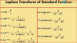
The standard functions and their corresponding Laplace transforms are:
- Constant Function: The Laplace transform of a constant function
f(t) = 1is given byF(s) = 1/s. - Polynomial Function: For the polynomial
f(t) = t^n, the transform isF(s) = n!/s^(n+1), where n! denotes factorial. - Exponential Function: The Laplace transform for the function
f(t) = e^(at)isF(s) = 1/(s-a). - Sine and Cosine Functions: For the sine function
f(t) = sin(at), the Laplace transform isF(s) = a/(s^2 + a^2), and for the cosine functionf(t) = cos(at), it isF(s) = s/(s^2 + a^2).
These transforms simplify complex differential equations, especially in engineering contexts like control systems, vibrations, and fluid dynamics. By converting differential equations into algebraic equations, the Laplace transform allows engineers to analyze and design systems more effectively.
Youtube Videos

Audio Book
Dive deep into the subject with an immersive audiobook experience.
Constant Function
Chapter 1 of 5
🔒 Unlock Audio Chapter
Sign up and enroll to access the full audio experience
Chapter Content
Function f(t)
1
Laplace Transform F(s)
1
s
Detailed Explanation
The Laplace transform of a constant function (f(t) = 1) leads to a simpler expression. To compute this, we replace f(t) with 1 in the Laplace transform definition:
L{1} = ∫[0 to ∞] e^(-st) * 1 dt.
This results in the integral that evaluates to 1/s, which is a standard result in Laplace transforms.
Thus, for a constant function of value 1, the Laplace transform results in 1/s.
Examples & Analogies
Imagine you are measuring a steady flow of water from a tap that constantly delivers 1 liter of water per second. In this scenario, the flow rate stays the same (constant at 1), and the Laplace transform helps to simplify any analysis of this constant flow over time.
Power Functions
Chapter 2 of 5
🔒 Unlock Audio Chapter
Sign up and enroll to access the full audio experience
Chapter Content
Function f(t)
tn
Laplace Transform F(s)
tn
sn+1
n!
Detailed Explanation
The Laplace transform of the function t raised to the power n, denoted as f(t) = t^n, results in F(s) = n!/s^(n+1). This arises from calculating the integral of t^n multiplied by the exponential decay e^(-st), leading us to the conclusion that for every increase in power, the Laplace transform introduces a factorial in the numerator and alters the growth of s in the denominator.
This shows how the Laplace transform dynamically adjusts the representation of different powers of t.
Examples & Analogies
Think of a car accelerating over time, where the distance traveled h(t) increases as a power function based on how long it has been accelerating (t^2). The Laplace transform helps to evaluate this distance in a simplified form, much like summarizing a complex journey in just a few numbers.
Exponential Functions
Chapter 3 of 5
🔒 Unlock Audio Chapter
Sign up and enroll to access the full audio experience
Chapter Content
Function f(t)
eat
Laplace Transform F(s)
eat
s−a
Detailed Explanation
For the exponential function f(t) = e^(at), the Laplace transform yields F(s) = 1/(s - a). This result arises from the special property of the exponential function, where the decay factor (s - a) adjusts based on the value of a, allowing us to capture the behavior of the function in various applications.
This makes exponential functions particularly useful, especially in engineering contexts like modeling growth or decay processes.
Examples & Analogies
Consider how populations grow over time, where the growth rate is constant (like e^(at)). By applying the Laplace transform, we can predict how long it will take for the population to reach a certain size, simplifying complex models into manageable predictions.
Sine Functions
Chapter 4 of 5
🔒 Unlock Audio Chapter
Sign up and enroll to access the full audio experience
Chapter Content
Function f(t)
sin(at)
Laplace Transform F(s)
a
s2+a2
Detailed Explanation
The Laplace transform of the sine function, f(t) = sin(at), results in F(s) = a/(s^2 + a^2). This can be derived from evaluating the integral of sin(at) multiplied by the exponentially decaying factor e^(-st). The behavior of the sine function is captured in this transformation, allowing it to be modeled effectively in various applications.
It's an elegant solution that enables the transformation from a time-dependent function into a frequency domain that engineers and scientists frequently use.
Examples & Analogies
Consider a swinging pendulum: its motion can be represented as a sine wave. The Laplace transform helps engineers analyze and predict the swing's behavior over time, converting the continuous motion into a form easily manipulated in calculations or simulations.
Cosine Functions
Chapter 5 of 5
🔒 Unlock Audio Chapter
Sign up and enroll to access the full audio experience
Chapter Content
Function f(t)
cos(at)
Laplace Transform F(s)
s
s2+a2
Detailed Explanation
Similar to the sine function, the Laplace transform for the cosine function f(t) = cos(at) results in F(s) = s/(s^2 + a^2). This outcome is derived through the integration of cos(at) while incorporating the exponential decay factor, showcasing the cosine wave's alternating behavior in a transformed manner.
This result is particularly useful in engineering fields, allowing for the handling of oscillatory systems effectively.
Examples & Analogies
Imagine a car moving smoothly down a curved road; its path can be modeled using a cosine function. The Laplace transform provides tools to analyze such curved trajectories scientifically, helping automotive engineers design safer and more efficient vehicles.
Key Concepts
-
Laplace Transform: A tool to convert time-domain functions into the s-domain, simplifying the solution of differential equations.
-
Standard Functions: Functions like constants, polynomials, exponentials, sines, and cosines that have known transforms.
Examples & Applications
The Laplace transform of f(t) = 1 is F(s) = 1/s.
For f(t) = t^2, the Laplace transform is F(s) = 2/s^3.
Memory Aids
Interactive tools to help you remember key concepts
Rhymes
If f(t) equals one, just run, F(s) = 1/s, that’s your fun!
Stories
Imagine a mathematician who could magically transform functions into s-space, making them easier to work with — that’s the magic of Laplace!
Memory Tools
For sine, remember: A (numerator) over (s^2 + a^2); for cosine, it’s s (numerator) over the same denominator — just remember 'A for A' and 's for s'!
Acronyms
CPE — Constants, Polynomials, Exponentials — the key standard functions with simple transforms!
Flash Cards
Glossary
- Laplace Transform
An integral transform that converts a function of time into a function of a complex variable, simplifying the analysis of linear time-invariant systems.
- Standard Functions
Common functions like constants, polynomials, exponentials, sine, and cosine used frequently in engineering mathematics.
- Region of Convergence
The range of values for which a Laplace transform converges and is valid.
Reference links
Supplementary resources to enhance your learning experience.