
Properties of Laplace Transforms
Enroll to start learning
You’ve not yet enrolled in this course. Please enroll for free to listen to audio lessons, classroom podcasts and take practice test.
Interactive Audio Lesson
Listen to a student-teacher conversation explaining the topic in a relatable way.
Linearity of Laplace Transforms
🔒 Unlock Audio Lesson
Sign up and enroll to listen to this audio lesson

Today, we will explore the linearity property of Laplace transforms, which states that the transform of a linear combination of functions equals the corresponding linear combination of their transforms.

Can you give an example of how that works?
Sure! If we have two functions, f(t) and g(t), and constants a and b, we can say: L{af(t) + bg(t)} = aL{f(t)} + bL{g(t)}. This means we can analyze each function separately and then combine the results.

So, we can break complex problems into simpler parts?
Exactly! And that's crucial in engineering applications where we often deal with composite systems.

What does this mean for differential equations?
It means we can transform the problem into parts that are easier to solve individually and later combine for the overall solution.
In summary, since L represents the Laplace transform, remember 'Linearity = L of linear combinations' simplifies our process!
First Shifting Theorem
🔒 Unlock Audio Lesson
Sign up and enroll to listen to this audio lesson

Now, let's discuss the First Shifting Theorem, which helps us to transform exponentially growing functions.

How does that theorem apply in real problems?
Great question! The theorem states that L{e^{at}f(t)} = F(s-a). It shifts the 's' value in the transform.
So, we can handle growth or decay in our functions using this?
Exactly. This is crucial in modeling systems affected by exponential growth, such as startup processes in engineering.
Can you summarize how to remember this theorem?
Remember, 'Shifting means a! Keep s in check with a!' This will help you keep the relationships in mind during problems.
Derivative Theorem
🔒 Unlock Audio Lesson
Sign up and enroll to listen to this audio lesson
Next, we have the Derivative Theorem, which allows us to take derivatives within the Laplace transform.
What does that look like in formula form?
It’s expressed as: L{d^n f(t)/dt^n} = s^n F(s) - s^{n-1}f(0) - ... - f^{(n-1)}(0). You see how initial conditions play a role?
Why is this important?
This property is critical for solving initial value problems where we need values at t = 0.
How can we easily remember all these terms?
You can remember, 'Derivatives + Laplace = Sidekicks!' This helps keep the derivative relationships front of mind.
Integration Theorem
🔒 Unlock Audio Lesson
Sign up and enroll to listen to this audio lesson
Finally, let's check out the Integration Theorem, which helps with integrating functions in the time domain.
What does that theorem state?
The theorem states: L{∫(0 to t) f(τ) dτ} = (1/s) F(s). This means we can manage accumulations effectively.
Are there situations in engineering where we'd use this?
Definitely! In systems where the response builds over time, like in dynamic load analysis.
How do I remember this?
'Integrate into Laplace, then multiply by s!' will help keep the relationship clear.
To summarize, we have learned - linearity simplifies compositions, shifting tackles growth, derivatives handle rate changes, and integration serves accumulation!
Introduction & Overview
Read summaries of the section's main ideas at different levels of detail.
Quick Overview
Standard
The properties of Laplace transforms include linearity, shifting theorems, derivative theorems, and integration theorems. These properties enhance the utility of Laplace transforms in solving initial value problems in engineering mathematics.
Detailed
Properties of Laplace Transforms
The properties of Laplace transforms play a crucial role in transforming complex differential equations into manageable algebraic expressions. The primary properties covered in this section are:
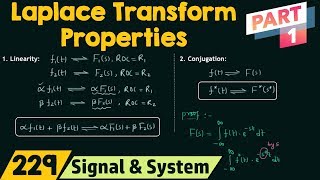
1. Linearity
The linearity property states that if you have linear combinations of functions, the transform can be distributed over these combinations:
$$L\{af(t)+bg(t)\} = aL\{f(t)\} + bL\{g(t)\}$$
This property allows the analysis of systems by breaking them down into simpler parts.
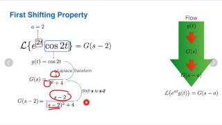
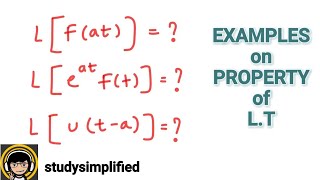
2. First Shifting Theorem
This theorem introduces a method to handle exponentially growing functions:
$$L\{e^{at}f(t)\} = F(s-a)$$
It is particularly useful when dealing with functions defined for t ≥ 0 that involve exponential growth or decay.
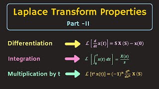
3. Derivative Theorem
The derivative theorem permits the handling of derivatives within the Laplace transform, catering to differential equations with initial conditions:
$$L\{\frac{d^n f(t)}{dt^n}\} = s^n F(s) - s^{n-1}f(0) - \ldots - f^{(n-1)}(0)$$
This is indispensable for solving initial value problems where conditions at t = 0 are known.
4. Integration Theorem
The integration theorem simplifies the process of integrating functions in the time domain:
$$L\{\int_{0}^{t} f(\tau) d\tau \} = \frac{1}{s} F(s)$$
This capability is vital for handling systems where accumulations of responses over time are necessary.
Together, these properties enable engineers and mathematicians to effectively utilize Laplace transforms in analyzing and solving ordinary differential equations that arise in real-world applications.
Youtube Videos

Audio Book
Dive deep into the subject with an immersive audiobook experience.
Linearity
Chapter 1 of 4
🔒 Unlock Audio Chapter
Sign up and enroll to access the full audio experience
Chapter Content
L{af(t)+bg(t)}=aL{f(t)}+bL{g(t)}
Detailed Explanation
The property of linearity states that the Laplace transform of a linear combination of functions can be calculated by applying the transform to each function separately and multiplying by their respective coefficients. In simpler terms, if you have two functions, f(t) and g(t), and you take their weighted sum (i.e., a times f(t) plus b times g(t)), the Laplace transform of this sum is equal to 'a times the Laplace transform of f(t)' plus 'b times the Laplace transform of g(t)'. This makes it straightforward to handle multiple functions within a single transform process.
Examples & Analogies
Imagine you are mixing different colors of paint. If you have a red paint (which represents f(t)), and a blue paint (which represents g(t)), the resulting color (the combination af(t) + bg(t)) can be achieved by mixing specific amounts of red and blue. Just like how you can calculate the resulting color using the amount of each color you have, you can calculate the Laplace transform of the mixed function by applying the transform individually to red and blue paints (or functions in this case).
First Shifting Theorem
Chapter 2 of 4
🔒 Unlock Audio Chapter
Sign up and enroll to access the full audio experience
Chapter Content
L{eatf(t)}=F(s−a)
Detailed Explanation
The First Shift Theorem indicates that if you multiply a function f(t) by an exponential function eat, the result of the Laplace transform is equivalent to taking the Laplace transform of f(t) and replacing the variable s with (s - a). This property is particularly useful in solving differential equations where the input is affected by an exponentially growing or decaying modifier.
Examples & Analogies
Consider a car accelerating at a constant rate (a) as opposed to moving at a constant speed. If you're measuring the total distance (the Laplace transform) while accounting for this acceleration, your measurements must adjust for the fact that the car is gaining speed. Instead of measuring the car's initial speed directly, you need to adjust your measurements to account for that extra speed due to acceleration, much like substituting (s - a) instead of just s.
Derivative Theorem
Chapter 3 of 4
🔒 Unlock Audio Chapter
Sign up and enroll to access the full audio experience
Chapter Content
L{d^n f(t)/dt^n} = s^n F(s) - s^{n-1}f(0) - ... - f(n-1)(0)
Detailed Explanation
The Derivative Theorem states that when you take the Laplace transform of the nth derivative of a function f(t), you can express this transform in terms of the Laplace transform of the original function F(s). The transformation incorporates both the 's' variable raised to the power of n and the initial conditions of the derivative function evaluated at zero. This is particularly useful in solving ordinary differential equations (ODEs) involving initial conditions, allowing us to easily compute the Laplace transform without differentiating the original function multiple times.
Examples & Analogies
Imagine you're tracking the position of a person walking down a street. The person’s position is the original function (f(t)), their speed is the first derivative (f'(t)), and their acceleration is the second derivative (f''(t)). If you want to analyze how far they have traveled over time, you can sum up their speed and alterations directly rather than continually measuring their position and change outside of their starting location. The equation helps connect the derivatives (speed, acceleration) back to the position in a straightforward way.
Integration Theorem
Chapter 4 of 4
🔒 Unlock Audio Chapter
Sign up and enroll to access the full audio experience
Chapter Content
L{∫(from 0 to t)f(τ)dτ} = F(s)/s
Detailed Explanation
The Integration Theorem states that if you take the Laplace transform of the integral of a function f(τ) from 0 to t, the result is simply the Laplace transform of that function divided by s. This property is useful when dealing with integrals as it allows for a straightforward calculation of the transform without needing to evaluate the integral explicitly.
Examples & Analogies
Think about how you measure the total amount of water in a swimming pool over time. As you fill it, the amount of water corresponds to the integral of the water flow over a period. If you know the flow rate (f(t)), instead of continuously measuring the water level, you can deduce the total water volume currently in the pool (the Laplace transform) by dividing the flow rate function by the time variable s. This makes calculating the total volume much simpler!
Key Concepts
-
Linearity: The property that allows transformations to be distributed over linear combinations of functions.
-
First Shifting Theorem: Facilitates handling exponential growth in functions within Laplace transforms.
-
Derivative Theorem: Handles the transformation of derivatives and integrates initial conditions into analysis.
-
Integration Theorem: Manages time-domain integrations effectively within transformations.
Examples & Applications
Using the linearity property, if L{f(t)} = F(s) and L{g(t)} = G(s), then L{2f(t) + 3g(t)} = 2F(s) + 3G(s).
Using the First Shifting Theorem, if f(t) = e^(2t), then L{e^(2t)f(t)} results in a shift: L{e^(2t)g(t)} = G(s-2).
Memory Aids
Interactive tools to help you remember key concepts
Rhymes
Linearity is a key, break it down, let it be!
Stories
Imagine a team of engineers solving a differential equation. They decide the best way is not to tackle it all at once - instead, they divide the work based on the linearity of each function.
Memory Tools
LDSI: Linearity, Derivatives, Shifting, Integration - Remember the key properties of Laplace!
Acronyms
LDS - for Linear, Derivative, and Shift properties in Laplace transforms.
Flash Cards
Glossary
- Linearity
The property allowing the Laplace transform to be distributed over linear combinations of functions.
- First Shifting Theorem
A theorem that states L{e^{at}f(t)} = F(s-a), facilitating the transform of exponentially growing functions.
- Derivative Theorem
The theorem allowing the transformation of derivatives, expressed as L{d^n f(t)/dt^n} = s^n F(s) - s^{n-1}f(0) - ... - f^{(n-1)}(0).
- Integration Theorem
The theorem that states L{∫(0 to t) f(τ) dτ} = (1/s) F(s) for managing time-domain integrations.
Reference links
Supplementary resources to enhance your learning experience.