
Estimation of Average Velocity in Pipe
Enroll to start learning
You’ve not yet enrolled in this course. Please enroll for free to listen to audio lessons, classroom podcasts and take practice test.
Interactive Audio Lesson
Listen to a student-teacher conversation explaining the topic in a relatable way.
Introduction to Average Velocity in Pipes
🔒 Unlock Audio Lesson
Sign up and enroll to listen to this audio lesson

Today, we’re covering the estimation of average velocity in pipes. Can anyone tell me what they understand by average velocity?

I think it's the typical speed that fluid flows through a pipe, but I guess it varies depending on the flow type.
Exactly! In turbulent flow, we often discuss something called 'velocity defects.' This refers to how much the actual flow velocity deviates from the average velocity. Think of it as a measure of how chaotic the flow is compared to the mean flow, like comparing the average classroom noise to a few loud students!

So, it’s kind of like when you’re trying to read in a noisy room, some parts are louder than the average?
Great analogy! Now, when analyzing such flows, we can express velocities mathematically using different dimensions. Can anyone recall the relationship we're focusing on?

Isn’t it linked to variables like height and distance from the pipe center?
Right! Understanding these relationships helps us visualize and calculate the flow behavior. Remember the acronym HALO to help recall: Height, Average velocity, Length, and Other factors.
To summarize, average velocity represents the mean speed of fluid flow, while velocity defects indicate variations. Keep these points in mind moving forward!
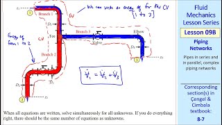
Pipes in Series
🔒 Unlock Audio Lesson
Sign up and enroll to listen to this audio lesson

Now let's discuss pipes in series. Why do you think the energy loss differs in these setups?

Isn’t it because the fluid has to flow through multiple pipes, each causing some resistance?
Exactly! The total head loss is the sum of individual head losses from each pipe. Remember that major losses from friction and minor losses from fittings and changes in diameter affect each segment.
So, if I had three pipes, I would add up the losses from each one to see the total loss?
Correct! Always consider both major and minor losses when calculating flow. A friendly reminder: use the acronym MAME for Major and Minor Energy losses!
Got it! We can quantify how these losses impact flow rates through the series.
Exactly! Summarizing, in a series setup, total head loss is cumulative, influenced by major and minor losses that affect energy efficiency in the system.
Pipes in Parallel
🔒 Unlock Audio Lesson
Sign up and enroll to listen to this audio lesson
Let's shift to parallel pipes. What do you think happens to the energy losses in this configuration?
Do they have to be equal across all paths because the flow is divided?
Exactly! In a parallel arrangement, all paths must face the same energy loss for flow to be distributed evenly. Remember, we use the term ENERGY EQUALIZATION here!
So if one pipe is smaller and has more resistance, it will still balance with larger ones?
Yes! Balancing determines the overall system efficiency. It’s like sharing the effort with a group; no single member can take on all the work!
To wrap up, in parallel pipes, ensure losses are balanced across pathways, maintaining overall system integrity.
Reservoir Junction Problems
🔒 Unlock Audio Lesson
Sign up and enroll to listen to this audio lesson
Now we’ll explore scenarios with reservoir junctions. Why is understanding junction flow crucial?
Because we need to know how much water can move between junctions?
Absolutely! Here, the Mass Conservation Principle applies. Can someone explain what that means?
It’s about ensuring that the total discharge in equals the total discharge out!
Exactly! At junctions, the sum of flows must equal zero, ensuring balance. Use the acronym MIND for Mass IN vs Mass OUT!
What if there are energy losses represented at these junctions?
Those must be accounted for in evaluating head losses. In conclusion, the flow through junctions is ultimately about balancing discharge and energy losses!
Practical Applications and Examples
🔒 Unlock Audio Lesson
Sign up and enroll to listen to this audio lesson
Let’s look at a real-life problem to apply what we've learned. Who can describe the basic setup of a given example?
It’s about a horizontal pipe with varying diameters and flow rate requirements?
Correct! Using the derived equations, can anyone calculate the required diameter for a specific head loss?
I think we’d set the losses equal between branches and solve for diameter?
Yes! It’s functional math entwined with physical flow principles. Remember that using theoretical examples solidifies understanding in practical contexts!
This makes the concepts much clearer; seeing them in a numerical example is helpful!
Great! In summary, applying theory to examples solidifies understanding and preparation for real-world scenarios.
Introduction & Overview
Read summaries of the section's main ideas at different levels of detail.
Quick Overview
Standard
The content explains the concept of average velocity and velocity defects in pipes, providing insights into how turbulence affects velocity distribution. It covers practical scenarios like pipes in series and parallel, energy losses, and introduces different equations and experimental setups relevant to understanding pipe flow.
Detailed
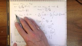
In this section, we delve into the estimation of average velocity in pipes, emphasizing key concepts such as velocity defects and the relationship between turbulence and average velocity. By utilizing dimensional analysis, we can estimate how far the velocity deviates from the average within the varying profiles of flow. Experimental data from the Nikuradse experiments indicate that a specific alpha value of 0.4 can be used to characterize velocity changes, especially in turbulent flows.
Further, the section explores practical applications, such as pipes arranged in series where energy losses combine linearly, and parallel pipes where energy losses must balance across multiple pathways. Each scenario underscores the importance of accounting for major and minor losses in assessing overall system performance. The logistics of reservoir junction problems are discussed, showcasing mass conservation principles and how to determine flow directions and energy loss across junctions.
By providing mathematical examples, including derivations from the Darcy-Weisbach equation, the section illustrates the process of estimating required gradients to maintain necessary flow rates under given conditions. Students learn to apply theoretical concepts to real-world scenarios, enhancing their understanding of fluid dynamics in piping systems.
Youtube Videos
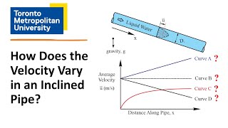

![Introduction to Velocity Fields [Fluid Mechanics #1]](https://img.youtube.com/vi/CkNo5xGMZS4/mqdefault.jpg)
Audio Book
Dive deep into the subject with an immersive audiobook experience.
Understanding Velocity Defects
Chapter 1 of 5
🔒 Unlock Audio Chapter
Sign up and enroll to access the full audio experience
Chapter Content
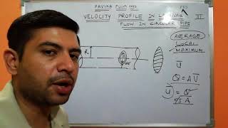
But if you go to the outer layers where we look it that a velocity defect concept, how far the velocity from average velocity, that the defect means how much deviations how much difference between that; if you look it that and looking, V = f(y, h)
Detailed Explanation
Velocity defects refer to the difference between the actual velocity of the fluid in the pipe and the average velocity. Understanding this concept involves looking closely at how fluid velocity varies within the layers of a pipe. The velocity can be expressed as a function of depth (y) and the height (h) of the fluid column. The outer layers of the fluid often have different velocities compared to the average due to turbulence and friction against the pipe walls.
Examples & Analogies
Think of it like a crowd of people walking through a narrow hallway. The people at the edges of the hallway are slowed down by the walls, while those in the center can move faster. The average speed of the crowd is slower than the speed of those in the center, just as the average velocity in a pipe might differ from the speed of fluid in the center.
High Turbulence and Velocity Profiles
Chapter 2 of 5
🔒 Unlock Audio Chapter
Sign up and enroll to access the full audio experience
Chapter Content
Now if you look it that, if you put it high turbulence flow and the velocity the reasons is very this is called velocity deflect law and h is replaced by the R the pipe radius then you can have this experimentally derived components and this alpha will represent a equal to the 0.4 and this is what the average velocity or time average velocity components and this is a special average velocity component how they are fluctuating with shear velocity.
Detailed Explanation
In cases of high turbulence flow, the average velocity can be significantly affected. The 'velocity defect law' describes how the average velocity is influenced by the turbulence. It uses the pipe radius (R) in the calculation, as this can indicate how quickly the fluid can move through the pipe. The constant 'alpha' is experimentally determined to be 0.4 in these scenarios, showing how the average (or time-average) velocity behaves alongside shear velocity—which is the rate at which layers of fluid slide past each other.
Examples & Analogies
Imagine a blender. When you blend liquids, the center spins quickly while the outer parts lag behind. The effective mixing speed you notice is like the average velocity, which may not reflect the actual speeds of all parts of the liquid due to turbulence.
Dimensional Analysis and Experimental Data
Chapter 3 of 5
🔒 Unlock Audio Chapter
Sign up and enroll to access the full audio experience
Chapter Content
And more details if in a overlap zones you will have a this equation. So now if you look it from the experiment and the dimensional analysis using this Nikuradse experiment data set it was found what could be the alpha value okay which is here is 0.4 and for the overlapped zones alpha, beta as a different value and here I am not talking much more. It is called the logarithmic overlap layers okay.
Detailed Explanation
In the study of fluid dynamics, experiments help determine how different parameters relate to each other. The 'Nikuradse experiment' specifically helps deduce values like alpha (0.4) in different flow conditions, especially in 'overlap zones.' These are regions where flow characteristics transition between different behaviors, and understanding them is crucial for accurate modeling of fluid flow.
Examples & Analogies
Consider a highway with two lanes merging into one. The traffic flow in the overlap zone behaves differently as cars slow down to fit into a single lane—this represents the complexity of layering and flow behavior at different velocities, similar to what happens in fluid flow within pipes.
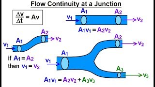
Pipe Flow Configurations: Series and Parallel
Chapter 4 of 5
🔒 Unlock Audio Chapter
Sign up and enroll to access the full audio experience
Chapter Content
Now we coming back to the very simple examples okay. And that is what is in your text book is necessary to for. If you look it that, many of the times you have the pipes in series, pipes in parallel or three reservoir junction problems okay.
Detailed Explanation
In civil and mechanical engineering, understanding how fluid flows through systems of pipes is essential. Pipes can be arranged in series (one after the other) or in parallel (next to each other). Each arrangement impacts fluid velocity and pressure. Analyzing these configurations helps engineers determine how efficiently fluids can be transported, based on continuity and energy loss equations.
Examples & Analogies
Think of water flowing through a garden hose system. If you have multiple hoses (pipes) connected—like one after another (series) or branching off (parallel)—the way water moves will change based on how they are set up, just like in engineered piping systems.
Energy Losses in Series and Parallel Pipes
Chapter 5 of 5
🔒 Unlock Audio Chapter
Sign up and enroll to access the full audio experience
Chapter Content
If you have definitely the discharge will be for a steady state conditions for steady flow conditions. So discharge at the Q1, Q2, Q3 that should be equal because this is a steady state. Q1 = Q2 = Q3 = constant
Detailed Explanation
In a steady flow system, the discharge (quantity of fluid flowing) remains constant across each connected pipe. This means that the flow entering any section of the pipe system must equal the flow at each subsequent section. When analyzing energy losses, it's essential to consider both major losses (friction) and minor losses (like changes in diameter), as they affect the total energy available for the flow.
Examples & Analogies
Imagine filling three connected buckets with water using one faucet. The amount of water flowing from the faucet must equal the combined amount flowing into all three buckets, assuming no leaks or spills—much like how fluid must maintain consistent discharge through pipe systems.
Key Concepts
-
Velocity Defect: A measure of how actual flow deviates from average velocity.
-
Energy Loss: Loss of energy mainly due to friction in pipes.
-
Head Loss: The decrease in total mechanical energy of the fluid due to friction and turbulence.
-
Major vs Minor Losses: Major losses account for friction; minor losses account for fittings and bends.
-
Reservoir Junction Problems: Focus on mass conservation at junction points in pipe networks.
Examples & Applications
Example of estimating energy loss in a pipe by applying major and minor loss concepts.
Example of a flow rate computation through multiple parallel pipes maintaining equal energy losses.
Memory Aids
Interactive tools to help you remember key concepts
Rhymes
In pipes that run so straight, losses in layers accumulate.
Stories
Imagine a farmer with a network of pipes in fields—each path needs to flow equally to ensure crops thrive, just like fluids through junctions.
Memory Tools
Remember 'M.I.N.D' for mass in equals mass out at junctions involving fluid flows.
Acronyms
Use 'HALO' - Height, Average velocity, Length, Other factors in calculating pipe dynamics.
Flash Cards
Glossary
- Average Velocity
The mean speed of fluid flow through a pipe.
- Velocity Defect
The deviation of actual fluid velocity from the average velocity.
- Energy Loss
The reduction of mechanical energy in the flow due to friction and other losses.
- Major Losses
Losses primarily due to friction in the pipe.
- Minor Losses
Losses due to fittings, changes in diameter, and other disturbances.
- Reservoir Junction
A point where multiple pipe flows converge or diverge.
Reference links
Supplementary resources to enhance your learning experience.