
Velocity Deflect Law
Enroll to start learning
You’ve not yet enrolled in this course. Please enroll for free to listen to audio lessons, classroom podcasts and take practice test.
Interactive Audio Lesson
Listen to a student-teacher conversation explaining the topic in a relatable way.
Understanding Velocity Defects
🔒 Unlock Audio Lesson
Sign up and enroll to listen to this audio lesson

Today, we'll be diving into the concept of velocity defects. Can anyone tell me what this term means?

Is it about how much the velocity of a fluid deviates from its average?
Exactly right, Student_1! Velocity defects describe how much the flow velocity differs from the average velocity, especially in turbulent flows. We use the notation 'V' for average velocity.

How do we actually measure or understand these deviations?
Great question! We use dimensional analysis and experimental data, like the Nikuradse experiments, to understand these relationships better.

What does turbulence have to do with this?
Turbulence causes fluctuations in velocity, leading to deviations we define as velocity defects. It’s crucial in designing effective fluid systems.
To remember the concept, think of 'VD' for Velocity Defect, representing the difference between average velocity and its fluctuating values.
In summary, velocity defects are essential in understanding flow dynamics in pipes, especially under turbulent conditions.
Energy Losses in Pipes
🔒 Unlock Audio Lesson
Sign up and enroll to listen to this audio lesson

Now that we understand velocity defects, let’s talk about energy losses when fluids flow through pipes. Who can explain what major and minor losses are?

Major losses are due to things like friction along the pipe, while minor losses happen due to fittings, changes in diameter, or entry/exit effects.
Correct, Student_4! It's important to compute both to understand overall energy loss. When pipes are in series, how do we calculate total head loss?
We sum all the head losses from each pipe, right?
Exactly! Each type contributes to total head loss, which is crucial in ensuring efficient flow through the system.
What about pipes in parallel?
Good point! In parallel configurations, energy losses must be equal across all paths. This ensures that the energy balance is maintained.
For a memory aid, remember 'PLE' - Parallel losses equalize. It reinforces that energy losses in parallel systems must match.
In summary, calculating energy losses due to major and minor sources is essential for managing fluid flow effectively in pipe systems.
Three Reservoir Junctions
🔒 Unlock Audio Lesson
Sign up and enroll to listen to this audio lesson
Lastly, let’s explore three reservoir junction problems. What do you think is special about these junctions?
They have multiple paths for flow, and we need to balance the discharges.
Great observation! The sum of all discharge at a junction must equal zero. Can you recall why?
Because of conservation of mass, right?
Exactly! This concept is crucial in ensuring that our systems are designed to manage flow effectively.
How do we actually determine the flow direction or head losses at these junctions?
We assess the hydraulic gradient lines and compute the energy losses at each direction to analyze flow paths.
For clarity, remember 'HGL' - Hydraulic Gradient Line. It will help you remember the importance of gradients in these junction analyses.
In conclusion, understanding the dynamics of three-reservoir junctions emphasizes the importance of mass conservation in fluid systems.
Introduction & Overview
Read summaries of the section's main ideas at different levels of detail.
Quick Overview
Standard
This section explains the primary concepts of the Velocity Deflect Law and its importance in analyzing fluid flow within pipes. It covers the significance of velocity defects, the effects of turbulence, and methods for calculating energy losses in various pipe systems.
Detailed
Velocity Deflect Law
The Velocity Deflect Law focuses on the concept of velocity defects, which indicate the deviations from the average velocity in turbulent flow. When examining the outer layers of fluid in a pipe, one can observe how velocity fluctuates relative to the average. The section details how to approach these fluctuations through dimensional analysis and experimental data, notably referencing the Nikuradse experiments. Key equations are introduced, such as those used to represent velocity distributions in turbulent flow.
In practical applications, the section illustrates the significance of calculating energy losses in scenarios involving pipes in series and parallel configurations. It explains how steady state flow ensures that the discharge remains constant across connected pipes while also navigating the differences in head loss due to various factors, such as friction and minor losses. Additionally, the concept of hydraulic gradient lines and the principles of mass conservation are emphasized, especially in the context of three-reservoir junction problems.
Through example problems, the section solidifies understanding by demonstrating how to compute minimum gradients necessary to maintain flow conditions and energy balance in fluid systems. Overall, the Velocity Deflect Law serves as a fundamental principle for analyzing flow dynamics in engineering applications.
Youtube Videos


Audio Book
Dive deep into the subject with an immersive audiobook experience.
Understanding Velocity Defect
Chapter 1 of 5
🔒 Unlock Audio Chapter
Sign up and enroll to access the full audio experience
Chapter Content
But if you go to the outer layers where we look at a velocity defect concept, how far the velocity from average velocity, that the defect means how much deviations how much difference between that.
Detailed Explanation
The velocity defect concept measures how far the actual velocity of a fluid differs from its average velocity. It focuses on the variations that occur, particularly in turbulent flow where these differences can be significant. This is important in fluid dynamics as deviations from average flow can influence efficiency and stability in systems.
Examples & Analogies
Imagine you are in a busy train station. The average flow of people is like the average velocity of a fluid. If many people take a detour or stop to chat (deviations), the flow becomes uneven, similar to how velocity fluctuations can affect overall fluid efficiency.
Dimensional Analysis in Velocity Measurement
Chapter 2 of 5
🔒 Unlock Audio Chapter
Sign up and enroll to access the full audio experience
Chapter Content
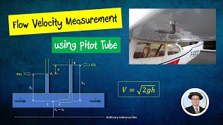
We again we get the similar functions from the dimensional analysis between V and y and h.
Detailed Explanation
Dimensional analysis helps in understanding the relationship between velocity (V), the distance from a reference point (y), and height (h). By analyzing these dimensions, we can create equations that describe how fluid behavior changes across different conditions. This fundamental understanding is crucial for predicting how changes in one parameter will influence the others in fluid dynamics.
Examples & Analogies
Consider you are trying to bake a cake. The relationship between flour (the base), sugar, and baking time can be understood through dimensional analysis. Just as using the right proportions affects the cake's outcome, understanding how velocity relates to distance and height helps predict fluid behaviors.
Velocity Deflect Law in Turbulent Flow
Chapter 3 of 5
🔒 Unlock Audio Chapter
Sign up and enroll to access the full audio experience
Chapter Content
Now if you look at high turbulence flow and the velocity the reasons is very this is called velocity deflect law and h is replaced by the R the pipe radius.
Detailed Explanation
The Velocity Deflect Law applies particularly in turbulent flow scenarios, where the dynamics and forces at play cause significant fluctuations in velocity. When analyzing these flows, the pipe radius (R) replaces height (h) in our calculations to better account for changes in the flow profile as it interacts with the pipe walls.
Examples & Analogies
Imagine a river rushing over rocks; the turbulence creates eddies and variations in speed. The pipe radius can be seen as the shape of the riverbed, influencing how water flows through and altering its speed and behavior.
The Role of Alpha in Velocity Components
Chapter 4 of 5
🔒 Unlock Audio Chapter
Sign up and enroll to access the full audio experience
Chapter Content
This alpha will represent a equal to the 0.4 and this is what the average velocity or time average velocity components...
Detailed Explanation
In analyzing turbulent flows, the coefficient alpha (often equaled to 0.4) becomes a crucial factor in calculating average velocities and their fluctuations over time. This value assists engineers and scientists in predicting how fluids behave under various scenarios, thereby improving designs and efficiencies in systems that utilize fluid transport.
Examples & Analogies
Think of alpha as the tuning fork for a musical note. Just like tuning ensures everyone in an orchestra plays harmoniously, understanding and applying alpha ensures that all calculations related to fluid motion are accurate and reliable.
Logarithmic Overlap Layers
Chapter 5 of 5
🔒 Unlock Audio Chapter
Sign up and enroll to access the full audio experience
Chapter Content
It is called the logarithmic overlap layers. Millikan gives the profile in the overlap zone...
Detailed Explanation
The logarithmic overlap layer refers to the region in a turbulent flow profile where the velocity gradients stabilize. In this layer, Millikan’s equation can be used to model the velocity distribution accurately, illustrating how fluid speed decreases as we move away from the wall of a pipe or channel.
Examples & Analogies
Imagine the way wind speed changes as you move away from a mountain. At first, it’s turbulent and chaotic close to the surface (high velocity), but becomes smoother and less powerful as you rise (gradually transitioning to lower velocity) – akin to the logarithmic overlap layers in fluid dynamics.
Key Concepts
-
Velocity Defect: Indicates deviations from average flow velocity in turbulent systems.
-
Energy Loss: Refers to the reduction in potential energy due to friction and other factors.
-
Hydraulic Gradient: The slope of pressure head vs. distance along a pipe.
-
Mass Conservation: The principle that mass cannot be created or destroyed in flow systems.
Examples & Applications
Calculating energy losses for a given diameter and flow rate in a series of connected pipes.
Determining the required pipe gradient to achieve a desired flow rate across a specified distance.
Memory Aids
Interactive tools to help you remember key concepts
Rhymes
In pipes the flow may tire, energy loss is quite dire.
Stories
Imagine a stream flowing smoothly, then hitting rough rocks. The energy lost is like friends losing their way, slowing down as they navigate the obstacles.
Memory Tools
Remember 'MD' for Major Loss and 'mD' for minor Losses, it keeps them side by side.
Acronyms
Think 'HGL' for Hydraulic Gradient Line; it shows how energy shifts in a fluid.
Flash Cards
Glossary
- Velocity Defect
The difference between instantaneous velocity and average velocity in a flow.
- Hydraulic Gradient Line (HGL)
A line that represents the hydraulic gradient of a fluid flow, showing potential energy changes.
- Major Loss
Energy losses primarily due to friction along a pipe.
- Minor Loss
Energy losses due to fittings, changes in pipe diameter, or entry/exit effects.
- Turbulent Flow
A flow regime characterized by chaotic changes in pressure and velocity.
Reference links
Supplementary resources to enhance your learning experience.