
Spectral Decomposition (For Symmetric Matrices)
Enroll to start learning
You’ve not yet enrolled in this course. Please enroll for free to listen to audio lessons, classroom podcasts and take practice test.
Interactive Audio Lesson
Listen to a student-teacher conversation explaining the topic in a relatable way.
Introduction to Spectral Decomposition
🔒 Unlock Audio Lesson
Sign up and enroll to listen to this audio lesson

Today, we'll explore spectral decomposition specifically for symmetric matrices. Can anyone explain what we mean by a symmetric matrix?

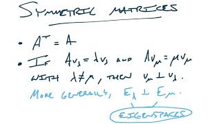
Isn't it a matrix that is equal to its transpose?
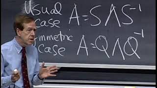
Exactly! Now, when we talk about spectral decomposition, we're expressing a symmetric matrix in this form: A = QΛQ^T. Who can tell me what each part represents?

Q is an orthogonal matrix and Λ is a diagonal matrix.
Good! The orthogonal matrix Q contains the normalized eigenvectors, while the diagonal matrix Λ holds the eigenvalues. This is crucial for operations like principal component analysis.

Why do we need the matrix to be symmetric?
Great question! Symmetric matrices guarantee real eigenvalues, facilitating their diagonalization. This leads us to our next point—the Spectral Theorem.

What does the Spectral Theorem state?
The Spectral Theorem states that every real symmetric matrix is diagonalizable by an orthogonal transformation. Remember this, as it applies widely across statistics and engineering!
In summary, spectral decomposition breaks down symmetric matrices into a product of matrices that simplify many calculations and analyses. Any questions?
Applications of Spectral Decomposition
🔒 Unlock Audio Lesson
Sign up and enroll to listen to this audio lesson

Now, let's discuss the applications of spectral decomposition. Why do you think it's important in principal component analysis?
Isn't it about reducing dimensionality by finding the main components that explain most of the variance?
Exactly! By diagonalizing the covariance matrix using spectral decomposition, we can identify these principal components efficiently. What about its application in mechanics?
It helps in analyzing stress and strain tensors, right?
Yes! Decomposing the stress tensor using eigenvalues and eigenvectors helps us understand the principal stresses and their orientations, essential for structural stability.
So, any symmetry in the stress tensor allows us to simplify and analyze its properties effectively?
Exactly! The symmetry ensures we have real eigenvalues, which helps us easily interpret the physical meaning of the results. Any final thoughts?
Mathematical Validation of Spectral Decomposition
🔒 Unlock Audio Lesson
Sign up and enroll to listen to this audio lesson
Alright, let’s delve into the math behind spectral decomposition. How do we prove that the eigenvector matrix Q is orthogonal?
Wouldn’t we need to show that Q^TQ equals the identity matrix?
Yes! And this holds true because eigenvectors corresponding to distinct eigenvalues of a symmetric matrix are orthogonal. What does this mean for our diagonal matrix Λ?
It implies that all off-diagonal elements are zero, right?
Correct! This makes the matrix easier to work with, especially in calculations like matrix exponentiation. Can anyone think of where we might need to perform such calculations?
In solving differential equations or in stability analysis!
Exactly! By utilizing spectral decomposition, we streamline complex calculations. Remember, this concept is not just theoretical but applicable in various engineering fields. Any questions on this validation process?
Introduction & Overview
Read summaries of the section's main ideas at different levels of detail.
Quick Overview
Standard
The section on spectral decomposition elaborates on how symmetric matrices can be expressed as products involving orthogonal matrices and diagonal matrices of their eigenvalues. Understanding this concept is crucial for applications in principal component analysis and stress analysis.
Detailed
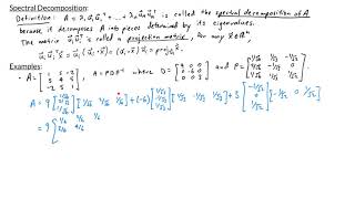
Spectral Decomposition of Symmetric Matrices
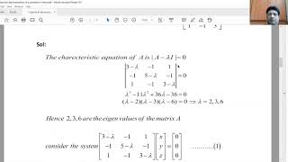
In linear algebra, spectral decomposition refers to the representation of a symmetric matrix as a product involving an orthogonal matrix and a diagonal matrix. For a symmetric matrix A in n-dimensional space, the spectral decomposition is expressed as:
A = QΛQ^T
Where:
- Q is an orthogonal matrix with columns representing the normalized eigenvectors of A.
- Λ is a diagonal matrix with eigenvalues λ₁, λ₂,..., λₙ on its diagonal.
The Spectral Theorem
This theorem states that any real symmetric matrix can be diagonalized through an orthogonal transformation. This property is essential, as it facilitates simplification in computations and enhances our understanding of the matrix's properties.
Applications of this theorem extend to various fields including statistics and engineering, especially in principal component analysis (PCA) and the decomposition of stress/strain tensors in mechanics.
Youtube Videos


Audio Book
Dive deep into the subject with an immersive audiobook experience.
Spectral Decomposition Formula
Chapter 1 of 2
🔒 Unlock Audio Chapter
Sign up and enroll to access the full audio experience
Chapter Content
If A∈Rn×n is symmetric, then:
A=QΛQT
Where:
• Q is an orthogonal matrix whose columns are normalized eigenvectors,
• Λ is a diagonal matrix with eigenvalues λ₁,...,λₙ.
Detailed Explanation
The section begins by introducing the concept of spectral decomposition specifically for symmetric matrices. The formula states that a symmetric matrix A can be expressed as a product of three matrices: Q, Λ, and the transpose of Q (QT). In this formula, Q represents an orthogonal matrix, meaning that its columns (which are the normalized eigenvectors of A) are orthogonal to each other and have unit length. Λ is a diagonal matrix that contains the eigenvalues of the matrix A along its diagonal. This implies that when we multiply these matrices together, we can reconstruct the original symmetric matrix A.
Examples & Analogies
Think of a symmetric matrix as a structure made from a set of forces acting in different directions. The orthogonal matrix Q is like a team of specialists, each one representing a specific direction (eigenvector) that the forces can act upon. The diagonal matrix Λ contains the strength of these forces (eigenvalues), determining how powerful each vector is in influence. When the specialists work together in the right way (through the multiplication of these matrices), they recreate the original system of forces perfectly.
Spectral Theorem
Chapter 2 of 2
🔒 Unlock Audio Chapter
Sign up and enroll to access the full audio experience
Chapter Content
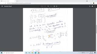
Spectral Theorem (Real Symmetric Case): Every real symmetric matrix is diagonalizable by an orthogonal transformation. This is fundamental in principal component analysis (PCA) and stress/strain tensor decomposition.
Detailed Explanation
The Spectral Theorem provides significant insight into real symmetric matrices. It states that any real symmetric matrix can be diagonalized through an orthogonal transformation. This means we can find an orthogonal matrix Q and a diagonal matrix Λ such that A can be expressed as A = QΛQT. Diagonalization simplifies complex calculations and makes it easier to analyze properties of matrices, such as eigenvalues and eigenvectors. The theorem is particularly important in applications like Principal Component Analysis (PCA), which is used to reduce the dimensionality of data, and in engineering fields for analyzing stress and strain tensors in materials.
Examples & Analogies
Consider the way we often summarize large amounts of data in simpler forms. For example, when we look at a dataset with many variables, we might condense it down to the few most important factors. This process is similar to what the Spectral Theorem does with matrices. It takes a complex relationship (the symmetric matrix) and helps us understand it better by breaking it down into simpler components (eigenvalues and eigenvectors) without losing the original information.
Key Concepts
-
Spectral Decomposition: The expression of a symmetric matrix as a product of matrices involving eigenvectors and eigenvalues.
-
Orthogonal Transformation: A transformation that preserves angles and distances, crucial for maintaining the properties of symmetric matrices during diagonalization.
-
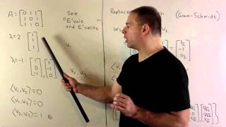
Real Symmetric Matrix: A type of matrix where all eigenvalues are real, and eigenvectors corresponding to distinct eigenvalues are orthogonal.
Examples & Applications
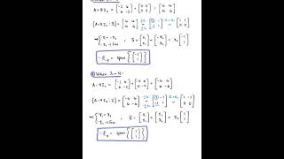
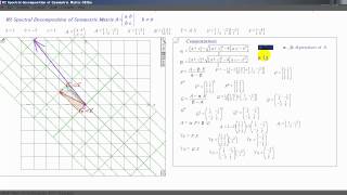
For a symmetric matrix A = [[2, 1], [1, 2]], the spectral decomposition yields A = QΛQ^T, where Q consists of the eigenvectors, and Λ contains the eigenvalues.
In principal component analysis, the covariance matrix of data is transformed via spectral decomposition to find the principal components efficiently, reducing dimensionality.
Memory Aids
Interactive tools to help you remember key concepts
Rhymes
To diagonalize and not to sweat, eigenvalues and vectors, don’t forget!
Stories
Imagine a team of explorers discovering a treasure. The treasure map is a matrix, and they need to find the true path (eigenvectors) and the value of the treasure (eigenvalues) through symmetry.
Memory Tools
Orthogonal Vectors Are Handy (OVAH) for keeping angles in check during decomposition!
Acronyms
PCA
Principal Components Analysis - Just remember it stands for breaking complexity down.
Flash Cards
Glossary
- Spectral Decomposition
Representation of a symmetric matrix as a product involving an orthogonal matrix and a diagonal matrix of its eigenvalues.
- Symmetric Matrix
A matrix that is equal to its transpose.
- Orthogonal Matrix
A square matrix whose columns and rows are orthogonal unit vectors.
- Eigenvector
A non-zero vector that changes at most by a scalar factor when a linear transformation is applied.
- Eigenvalue
A scalar that is associated with a linear transformation represented by an eigenvector.
- Diagonal Matrix
A matrix in which the entries outside the main diagonal are all zero.
- Principal Component Analysis (PCA)
A statistical technique used to simplify data by reducing its dimensionality.
Reference links
Supplementary resources to enhance your learning experience.