
Flow Profiles in Pipes
Enroll to start learning
You’ve not yet enrolled in this course. Please enroll for free to listen to audio lessons, classroom podcasts and take practice test.
Interactive Audio Lesson
Listen to a student-teacher conversation explaining the topic in a relatable way.
Kinetic Energy Correction Factors
🔒 Unlock Audio Lesson
Sign up and enroll to listen to this audio lesson

Welcome everyone! Today, we'll start with kinetic energy correction factors. Can anyone tell me why we need a correction factor in fluid mechanics?

Is it because the velocity isn't the same across the entire cross-section of a pipe?
Exactly! In real flows, due to varying velocities, we can't just use the average velocity to calculate kinetic energy directly. This is where our correction factor, alpha, comes into play. Remember, for laminar flow, the alpha is typically about 2. Can anyone remind me what the alpha values are for turbulent flow?

They range from about 1.04 to 1.11, don't they?
Right! Well done. This factor is crucial for accurate calculations in engineering applications. To remember this, think of the acronym 'KFC' for Kinetic Factor Correction.

That's a cool way to remember it! So, we really need to consider these factors when designing pipe systems, right?
Absolutely! Anytime you deal with pipes, factoring in these correction values is essential for precision. Let's summarize: kinetics in unsteady flow requires correction due to the non-uniform distribution of velocities.
Types of Pressure
🔒 Unlock Audio Lesson
Sign up and enroll to listen to this audio lesson

Next, let's dissect the three types of pressure. Who can explain what static pressure is?
Isn't static pressure the force exerted by a fluid at rest?
Correct! Now, what about dynamic pressure?
That's the pressure due to the fluid's motion, right?
Exactly! And when you add static and dynamic pressures together, what do you get?
Stagnation pressure!
Wonderful! To recall these concepts, think of the phrase 'Stay Daring and Stagnate'—each keyword hints at a pressure type.

That helps a lot! So all three types are essential for flow measurement?
Yes! They are vital for accurately describing and managing fluid behavior. In summary: static pressure reflects rest, dynamic pressure shows motion, and stagnation pressure combines both.
Energy Gradient Lines and Hydraulic Gradient Lines
🔒 Unlock Audio Lesson
Sign up and enroll to listen to this audio lesson
Now let's delve into energy and hydraulic gradient lines. Can anyone tell me what an energy gradient line represents?
It shows the total energy in the fluid, including kinetic, static, and potential energy?
Spot on! And what about the hydraulic gradient line?
It only considers the pressure and elevation heads.
Right again! The energy gradient line is broader, encompassing all forms of energy. To help remember, use 'Energize and Hydrate!'—since we want to manage both energy and pressures.
These lines are useful for pipeline designs, right?
Absolutely! They help engineers ensure fluid flows efficiently. To wrap up: Energy gradient lines consider total energy, while hydraulic gradient lines focus on pressures.
Applications of Bernoulli's Equation
🔒 Unlock Audio Lesson
Sign up and enroll to listen to this audio lesson
Let's discuss how we apply Bernoulli's equation through devices like orifice meters and venturimeters. What roles do these devices play?
They measure fluid flow rates, right?
Exactly! Orifices create a pressure drop, allowing us to quantify discharge. What about energy losses while using these devices?
Aren't they significant? We need to account for that with a coefficient of discharge.
Correct again! This coefficient helps bridge theoretical and actual discharge values. To remember: 'Cooperate in Discharge'—think of the coefficient helping in accurate calculations.
So combining theory with actual measurements is essential in engineering.
Absolutely! Insight into practical applications grounds our understanding of theory. In summary: Bernoulli's equation aids in designing efficient fluid systems using devices like orifice meters.
Introduction & Overview
Read summaries of the section's main ideas at different levels of detail.
Quick Overview
Standard
In this section, the flow profiles in pipes are explored through the lens of the Bernoulli equation, highlighting concepts like kinetic energy correction factors, pressure types, energy gradient lines, and practical applications including the use of orifice and venturimeter devices for measuring fluid flow.
Detailed
Flow Profiles in Pipes
This section delves into the critical aspects of fluid flow within pipes, anchored by the application of the Bernoulli equation. It begins with a brief overview of how the Bernoulli equation serves as a fundamental tool in fluid mechanics, providing insights into fluid behavior across various applications. Key topics include:
- Kinetic Energy Correction Factors: Understanding that fluid flow isn't uniform, this concept addresses corrections needed when applying average velocities to compute kinetic energy. In laminar flow conditions, the flow tends to be parabolic, while turbulent flow presents a logarithmic profile. The mention of correction factors (alpha values) highlights the complexity of accurately assessing energy in real fluid systems.
- Types of Pressure: This section further distinguishes between static, dynamic, and stagnation pressures, explaining how each plays a role in analyzing fluid behavior. The static pressure measures the pressure exerted by a fluid at rest, dynamic pressure involves the kinetic energy of the fluid, and stagnation pressure combines both when a fluid is brought to rest.
- Energy and Hydraulic Gradient Lines: The distinction between energy gradient lines (which encompass all energy forms: flow, kinetic, and potential) and hydraulic gradient lines (which consider only pressure and elevation head) is introduced. Understanding these lines enhances the ability to visualize and analyze energy changes within pipe flows.
- Applications: Practical applications of the Bernoulli equation are discussed through experimental setups involving venturimeters and orifice meters. These devices measure fluid discharge while accounting for energy loss within the systems, emphasizing the application of the coefficient of discharge (C_d) to quantify these discrepancies.
This section ultimately illustrates how well-structured applications of the Bernoulli equation can greatly inform the management of fluid flow in various engineering contexts.
Youtube Videos


Audio Book
Dive deep into the subject with an immersive audiobook experience.
Understanding Flow Profiles
Chapter 1 of 4
🔒 Unlock Audio Chapter
Sign up and enroll to access the full audio experience
Chapter Content
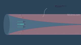
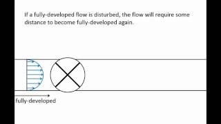
When discussing fluid flow through a pipe, it's essential to understand that the velocity distribution within the pipe is not uniform. This non-uniformity can manifest in two primary flow types: laminar and turbulent. Laminar flow is characterized by smooth and orderly layers of fluid, whereas turbulent flow involves chaotic and irregular movements.
Detailed Explanation
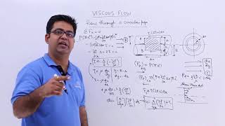
Flow profiles in pipes can be categorized mainly into two types: laminar and turbulent. In laminar flow, the fluid moves in parallel layers, and the velocity is highest in the center of the pipe, creating a parabolic profile. In contrast, turbulent flow exhibits a more chaotic behavior, leading to a more complex velocity distribution. Understanding these profiles is crucial because they affect how fluid behaves under different conditions, influencing calculations of velocity, pressure drops, and energy losses.
Examples & Analogies
Imagine a well-organized line of students (laminar flow) walking calmly in a hallway versus a chaotic crowd of students (turbulent flow) milling about before school. In the calm line, everyone moves smoothly and at a consistent pace, while in the crowd, people bump into each other and move erratically. This analogy helps illustrate the differences in flow types in pipes.
Kinetic Energy Correction Factors
Chapter 2 of 4
🔒 Unlock Audio Chapter
Sign up and enroll to access the full audio experience
Chapter Content
Due to the non-uniform velocity distribution in pipe flow, it's difficult to accurately compute kinetic energy using average velocity alone. Therefore, we introduce kinetic energy correction factors, also known as alpha (α). These factors adjust the calculated kinetic energy to account for the variations in velocity.
Detailed Explanation
In fluid mechanics, when we compute kinetic energy in a flow, we typically use the average velocity. However, since the velocity distribution is not uniform, this average may not accurately reflect the true kinetic energy of the fluid. The kinetic energy correction factor (α) helps us to rectify this issue. It allows us to scale the kinetic energy computed using average velocity to account for variations in velocity throughout the flow profile, leading to a more accurate representation of the energy present in the fluid.
Examples & Analogies
Consider a garden hose. If you measure the speed of water at the center, you might think all the water flows at that same speed. But water along the edge moves slower due to friction with the hose. Using the average measurement without adjustment can misrepresent how much energy the water actually has. The kinetic energy correction factor helps 'correct' that initial measurement, much like understanding that not all water flows in the same way.
Bernoulli Equation and Energy Gradients
Chapter 3 of 4
🔒 Unlock Audio Chapter
Sign up and enroll to access the full audio experience
Chapter Content
The Bernoulli equation expresses the relationship between pressure, velocity, and height in a fluid flow. Along a streamline, the total mechanical energy is conserved. This relationship helps define crucial elements like the energy gradient line and the hydraulic gradient line.
Detailed Explanation
Bernoulli's equation illustrates that in an ideal fluid flow, the sum of pressure energy, kinetic energy, and potential energy remains constant along a streamline. This principle leads to the concept of the energy gradient line, which represents the total mechanical energy of the fluid as it flows. The hydraulic gradient line, on the other hand, only takes into account the static pressure and elevation heads. Understanding these lines is critical for analyzing fluid flow in various applications, such as pipe systems and open-channel flows.
Examples & Analogies
Think of a roller coaster: at the top of a hill, the cars have maximum potential energy due to their height. As they descend, that potential energy converts into kinetic energy, making them speed up. The conservation of energy principle is similar in fluid mechanics, where we can visualize the flow of the fluid as a roller coaster, moving between energy states as it travels through the pipe system.
Application in Pipe Flow Design
Chapter 4 of 4
🔒 Unlock Audio Chapter
Sign up and enroll to access the full audio experience
Chapter Content
In practical applications, engineers must consider the energy gradient and hydraulic gradient lines in designing efficient pipe flows. The energy gradient shows how energy behaves along the flow, and understanding hydraulic gradient helps ensure that the pressure is adequate for maintaining flow.
Detailed Explanation
When designing piping systems, engineers utilize the energy gradient and hydraulic gradient lines to predict how energy changes along the flow and to ensure the pressure at various points in the system is sufficient to maintain the intended flow rate. Analyzing these gradients helps to identify potential issues such as areas where the pressure might drop too low, leading to cavitation or flow interruptions, which are critical for system reliability and efficiency.
Examples & Analogies
Imagine planning a road trip. If you know the roads (flow) have steep hills (energy gradients), you need to ensure your car (pressure) has enough fuel (energy) to reach the destination. Similarly, engineers need to assess the gradients in a pipe system to ensure that fluid maintains the right pressure and flow, avoiding potential problems like blockages or bursts in the pipeline.
Key Concepts
-
Kinetic Energy Correction Factor: Adjusts kinetic energy calculations for non-uniform velocity distributions in fluid flow.
-
Types of Pressure: Includes static, dynamic, and stagnation pressures critical for fluid mechanics.
-
Energy Gradient Line (EGL): Represents total energy in a fluid system, crucial for analyzing flow.
-
Hydraulic Gradient Line (HGL): Reflects static pressure and elevation, essential for fluid flow management.
-
Coefficient of Discharge (C_d): Expresses the efficiency of fluid flow measurement devices like orifices.
Examples & Applications
Using an orifice meter to measure water flow, calculating pressure drops, and determining the coefficient of discharge.
Designing a piping system that accounts for varying kinetic energy profiles using correction factors.
Memory Aids
Interactive tools to help you remember key concepts
Rhymes
In pipes where fluids flow so free, remember KFC for energy!
Stories
Imagine a river where the surface is smooth; that's static pressure, calm and soothed. A fish jumps high, creating dynamic change; together they stagnate, it's a fluid exchange.
Memory Tools
Keep your Sights on D for Stagnation, 'cause Dynamic's just one part of the Equation.
Acronyms
KDC for Kinetic, Dynamic, and Coefficient to remind you of pressures in motion.
Flash Cards
Glossary
- Kinetic Energy Correction Factor (α)
A factor used to adjust the kinetic energy calculations in fluid flow due to non-uniform velocity profiles.
- Static Pressure
The pressure exerted by a fluid at rest.
- Dynamic Pressure
The pressure associated with the fluid's motion.
- Stagnation Pressure
The pressure of a fluid when it is brought to rest, a combination of static and dynamic pressures.
- Energy Gradient Line (EGL)
A line representing the total energy of fluid flow, including kinetic and potential energies.
- Hydraulic Gradient Line (HGL)
A line that represents the static pressure and elevation head in fluid flow.
- Coefficient of Discharge (C_d)
The ratio of actual discharge to theoretical discharge through an orifice or venturimeter.
Reference links
Supplementary resources to enhance your learning experience.