
Kinetic Energy Correction Factors in Different Flows
Enroll to start learning
You’ve not yet enrolled in this course. Please enroll for free to listen to audio lessons, classroom podcasts and take practice test.
Interactive Audio Lesson
Listen to a student-teacher conversation explaining the topic in a relatable way.
Introduction to Fluid Flow
🔒 Unlock Audio Lesson
Sign up and enroll to listen to this audio lesson

Today, we will discuss how kinetic energy correction factors are essential in fluid mechanics, particularly when we deal with different flow profiles. Can anyone tell me what kinetic energy is?

Isn't it the energy that a body possesses due to its motion?
Exactly! Kinetic energy is given by the formula 1/2 mv². However, in fluid mechanics, the challenge arises when we use average velocities for flow calculations. Let's explore how flow isn't always uniform!

What happens to the kinetic energy if the flow doesn't have a uniform velocity?
Good question! When flow profiles vary, we need to use kinetic energy correction factors, typically denoted as alpha. This factor helps adjust the kinetic energy calculations to account for velocity variations.
Let's remember: K-E-C-F—Kinetic Energy Correction Factor! This acronym will help you remember its importance!
Understanding Flow Profiles
🔒 Unlock Audio Lesson
Sign up and enroll to listen to this audio lesson

Let's dissect the types of flow profiles. Who can explain the difference between laminar and turbulent flow?

Laminar flow is smooth and ordered, while turbulent flow is chaotic and mixed.
That's right! Laminar flows have a parabolic velocity profile, whereas turbulent flows exhibit a more complex pattern. In our calculations, we have different correction factors for both types. Can anyone guess what the α values might be?

For laminar flow, is it around 2?
Correct! And for turbulent flow, it generally varies between 1.04 to 1.1. It's crucial to apply these values correctly for accurate calculations in real-world applications.
Application of Correction Factors
🔒 Unlock Audio Lesson
Sign up and enroll to listen to this audio lesson
Now that we understand the importance of kinetic energy correction factors, how would we apply these in a flow case?
We need to find the actual kinetic energy using the average velocity and then multiply by the correction factor?
Exactly! When we compute kinetic energy based on average velocity, we consider the non-uniform distribution by applying alpha. So, the total kinetic energy can be expressed as KE_total = α * (1/2 ρV_average²), where α accounts for the actual flow behavior.
Can we calculate it for both laminar and turbulent cases together?
Yes, indeed! That is how engineers ensure accuracy in designs, especially when comparing different flow scenarios. Remember, understanding these corrections is vital for practical engineering applications!
Introduction & Overview
Read summaries of the section's main ideas at different levels of detail.
Quick Overview
Standard
The section discusses the significance of kinetic energy correction factors in determining the actual kinetic energy in fluid flows, especially when velocities vary from laminar to turbulent. It highlights how these factors correct the discrepancies that arise when using average velocities and provides equations for calculating kinetic energy based on flow characteristics.
Detailed
In fluid mechanics, the concept of kinetic energy correction factors is critical for accurately determining the kinetic energy of a flowing fluid. When fluid flows through a pipe or channel, it does not have a uniform velocity distribution. Instead, velocity tends to vary due to factors like viscosity and flow turbulence, resulting in complex flow profiles. This section elaborates on how to compute total kinetic energy using average velocities and integrates the concept of kinetic energy correction factors, denoted by alpha (α), which adjust the energy calculations to account for these non-uniformities. For laminar flow, α is typically around 2, while for turbulent flow, it ranges from 1.04 to 1.1. These correction factors ensure that engineers can design and analyze fluid systems with greater accuracy by aligning theoretical calculations with observed behaviors.
Youtube Videos


Audio Book
Dive deep into the subject with an immersive audiobook experience.
Uniform vs Non-Uniform Flow
Chapter 1 of 4
🔒 Unlock Audio Chapter
Sign up and enroll to access the full audio experience
Chapter Content
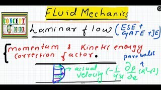
In fluid flow problems, the velocity distributions are often non-uniform. Flow can be laminar, creating a parabolic velocity profile, or turbulent, producing a logarithmic profile. This variation complicates the calculation of kinetic energy, as a simple average velocity does not represent the actual kinetic energy accurately.
Detailed Explanation
When fluids flow, the speed of the fluid can change depending on where you measure it inside the pipe or channel. If the flow is laminar, like a smooth and orderly stream, the speeds might create a parabolic shape when graphed. In contrast, turbulent flow, which is chaotic and irregular, creates a more complex, logarithmic shape. Because of these differences, using a simple average speed can lead to errors in calculating how much kinetic energy is present in the flow. To accommodate these variations, we need a correction factor.
Examples & Analogies
Imagine you are measuring the speed of runners in a race. If most runners are bunched together, knowing just the average speed won't help you understand who is winning. Some runners may be much faster or slower at different points on the track. Similarly, in fluid flow, knowing the average speed doesn’t give you the whole picture due to the differences in speeds at various points.
Kinetic Energy Correction Factor (α)
Chapter 2 of 4
🔒 Unlock Audio Chapter
Sign up and enroll to access the full audio experience
Chapter Content
To accurately account for this non-uniformity in flow, a kinetic energy correction factor (α) is introduced. The idea is to adjust the kinetic energy calculation when using average velocity instead of the varying velocity profile.
Detailed Explanation
The kinetic energy correction factor (α) is a multiplier that adjusts the kinetic energy calculated using the average velocity so that it reflects the real kinetic energy present due to the flow's speed variability. For laminar flow, this factor is typically 2, meaning that the kinetic energy calculated with the average velocity will need to be doubled to reflect the actual kinetic energy. For turbulent flow, α ranges from 1.04 to 1.11, indicating a slight increase over the average velocity's calculation. Therefore, this correction factor allows for a more accurate representation of the kinetic energy in non-uniform flow.
Examples & Analogies
Think of α like a recipe adjustment. If you're making a cake and the recipe says to use 2 cups of flour but you realize you need more because your flour isn’t as fluffy as the recipe assumed, you might need to adjust to 2.5 cups instead. In fluid dynamics, α is the adjustment we make because the standard formula doesn't fit our situation perfectly due to variations in flow speed.
Calculating α for Different Flows
Chapter 3 of 4
🔒 Unlock Audio Chapter
Sign up and enroll to access the full audio experience
Chapter Content
For fully developed laminar flow, the value of α is approximately 2. In turbulent pipe flow, α typically ranges from 1.04 to 1.11. It's crucial to calculate α accurately for fluid mechanics problems.
Detailed Explanation
In specific flow conditions, α can be determined with relative ease. For laminar flow, experiment shows us that the adjustment factor is consistently around 2, signifying that the average speed underestimates the actual kinetic energy. For turbulent flows, tests show that α fluctuates between 1.04 and 1.11, meaning the average flow speed gives a fairly close but slightly lower estimation of kinetic energy. Understanding these values is essential for accurately applying Bernoulli’s equation.
Examples & Analogies
Imagine you’re a coach timing the fastest runners in your team. The ones with better technique may frequently run the laps faster than the average times suggest. Just like the coach adjusts his strategies based on the athletes’ individual performances, engineers adjust their calculations using α to ensure safety and performance in their fluid systems.
Importance of Kinetic Energy Correction Factor
Chapter 4 of 4
🔒 Unlock Audio Chapter
Sign up and enroll to access the full audio experience
Chapter Content
Ignoring the kinetic energy correction factor can lead to significant errors in engineering calculations and the design of systems involving fluid flow.
Detailed Explanation
If engineers fail to include the kinetic energy correction factor in their calculations, they risk miscalculating the energy available to the fluid, which could lead to inadequate designs. This can affect everything from pipes and ducts to pumps and turbines, potentially leading to system failures, inefficiencies, or increased costs.
Examples & Analogies
It's similar to planning a budget without considering all expenses accurately. If a family underestimates their monthly expenses by not accounting for variable costs, they might find themselves short on funds. In the same way, failing to account for variable flow conditions in fluid systems can lead to underperformance or failures.
Key Concepts
-
Kinetic Energy Correction Factor (α): A key component in fluid mechanics that adjusts kinetic energy calculations for non-uniform velocity distributions.
-
Laminar Flow Characterization: Refers to the orderly movement of fluid with a parabolic profile.
-
Turbulent Flow Characteristics: Defined by chaotic fluid movement and a more complex velocity profile.
Examples & Applications
Example 1: A pipe with laminar flow has a velocity of 3 m/s and a calculated average kinetic energy of 4.5 J/kg. The correction factor α is applied to reflect the flow's actual behavior, resulting in a total kinetic energy computation of 9 J/kg.
Example 2: For turbulent flow in a channel with an average velocity of 2 m/s, and an α of 1.07, the kinetic energy would be correctly calculated, ensuring that real-world applications reflect these dynamics.
Memory Aids
Interactive tools to help you remember key concepts
Rhymes
Flow so smooth, a parabolic groove, laminar's the calm while turbulent's the storm.
Stories
Imagine a river where fish swim gracefully in layers, that's laminar flow, while in the rapids, they swirl in chaos—turbulent flow.
Memory Tools
K-E-C-F for Kinetic Energy Correction Factor—Correcting flows that don't act as a normal vector.
Acronyms
REMEMBER
K-E-C-F—Kinetic Energy Correction Factors for flow!
Flash Cards
Glossary
- Kinetic Energy Correction Factor (α)
A factor used to adjust kinetic energy calculations to account for non-uniform velocity distributions in fluid flow.
- Laminar Flow
A flow regime characterized by smooth and orderly motion of fluid particles, typically having a parabolic velocity profile.
- Turbulent Flow
A flow regime characterized by chaotic and irregular fluid motion, often resulting in a more complex velocity profile.
- Velocity Profile
A graphical representation of the distribution of fluid velocity across a cross-section of a flow.
- Average Velocity
The mean velocity of fluid across a given cross-section, calculated by integrating the velocity profile.
Reference links
Supplementary resources to enhance your learning experience.