
Applications of Bernoulli's Equation
Enroll to start learning
You’ve not yet enrolled in this course. Please enroll for free to listen to audio lessons, classroom podcasts and take practice test.
Interactive Audio Lesson
Listen to a student-teacher conversation explaining the topic in a relatable way.
Understanding Bernoulli's Equation
🔒 Unlock Audio Lesson
Sign up and enroll to listen to this audio lesson

Today we explore the applications of Bernoulli's Equation! How many of you can tell me what Bernoulli's Equation relates?

It connects pressure, velocity, and elevation, right?
Exactly! And when we consider real fluids, we often need to apply correction factors. What do we think the kinetic energy correction factor accounts for?

It adjusts for non-uniform flow conditions, right?
Correct! It’s crucial when we measure flow through devices like orifice meters. Can anyone explain what an orifice meter does?

It's used to measure the flow rate through a pipe by creating a pressure difference when fluid passes through an opening.
Well said! The relationship we derive also includes calculating the discharge using the coefficient of discharge. Let's remember: 'Theoretical Discharge is often higher than Actual Discharge because of losses!' Excellent work!
Types of Pressure
🔒 Unlock Audio Lesson
Sign up and enroll to listen to this audio lesson

Next, let's dive into pressure types! What can anyone tell me about static pressure?

It's the pressure exerted by a fluid at rest.
That's right! Now, how does static pressure relate to dynamic pressure?
Dynamic pressure is related to the motion of the fluid, like the kinetic energy from velocity.
Exactly! And combining both gives us stagnation pressure. If we have a pitot tube measuring stagnation pressure, what does it imply?
It measures the total pressure at a point where the fluid completely stops.
Correct! Remember: 'Static Pressure + Dynamic Pressure = Stagnation Pressure.' Good job, everyone!
Energy and Hydraulic Gradient Lines
🔒 Unlock Audio Lesson
Sign up and enroll to listen to this audio lesson
Let's talk about energy and hydraulic gradient lines. Who can define these lines and their significance?
The energy gradient line represents the total energy head, while the hydraulic gradient line excludes kinetic energy.
Exactly! And why do we draw these lines?
To visualize energy changes and understand where the fluid is likely to flow!
Right on! 'Fluid flows from high energy to low energy.' Very important to keep in mind!
Introduction & Overview
Read summaries of the section's main ideas at different levels of detail.
Quick Overview
Standard
The section delves into practical applications of Bernoulli's Equation in fluid mechanics, including orifice meters, venturi meters, and the impact of kinetic energy correction factors. It covers the definition of static, dynamic, and stagnation pressures, as well as hydraulic and energy gradient lines, illustrating their relevance in real-world scenarios such as automobile design and fluid flow systems involving pumps and turbines.
Detailed
In-Depth Summary of Applications of Bernoulli's Equation
The applications of Bernoulli's Equation are paramount in solving real fluid flow problems, significantly influencing industries such as automotive design and hydraulic engineering. Established by Daniel Bernoulli in 1752, this equation simplifies the analysis of fluid dynamics by providing a relationship between pressure, velocity, and elevation in a fluid stream. To effectively apply this equation in various contexts, certain concepts and adjustments are essential:
Key Concepts:
- Real Fluid Flow Problems: The fundamental utility of Bernoulli's Equation is its ability to model real fluid flows by incorporating correction factors for non-uniformity, such as kinetic energy correction factors. As fluid flows through various devices like orifice and venturi meters, understanding these corrections becomes crucial for accurate discharge measurements.
- Types of Pressures: The three distinct pressures defined are static pressure, dynamic pressure (or velocity head), and stagnation pressure (sum of the previous two). These pressures are instrumental in calculating fluid flow characteristics and understanding forces acting within fluid environments.
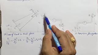
- Energy Gradient Line & Hydraulic Gradient Line: Both gradient lines visualize the energy perspectives across a fluid system. The energy gradient line represents the total energy including potential, kinetic, and pressure energy, while the hydraulic gradient line excludes the kinetic energy, simplifying certain calculations but still providing crucial insights into fluid behavior.
The applications extend through numerous scenarios, including the design of fuel-efficient vehicles, where optimizing drag coefficients has significantly improved consumption rates. Moreover, practical experiments conducted using orifice meters instantiate the application of Bernoulli's principles, illuminating the inherent energy losses versus calculated theoretical values through the understanding of coefficients of discharge.
Ultimately, Bernoulli's Equation and its applications remain a cornerstone in fluid mechanics, accomplishing practical, efficient solutions in engineering disciplines today.
Youtube Videos


Audio Book
Dive deep into the subject with an immersive audiobook experience.
Introduction to Bernoulli's Equation Applications
Chapter 1 of 9
🔒 Unlock Audio Chapter
Sign up and enroll to access the full audio experience
Chapter Content
I will start with the applications, very interesting applications I will show to you, then I will go for orifice meter experiment in IIT, Guwahati, then I will talk about kinetic energy corrections factors.
Detailed Explanation
This chunk introduces the various applications of Bernoulli's equation. The lecturer mentions starting with general applications, followed by specific experiments, and then discussing kinetic energy correction factors which adjust calculations for non-uniform flow distributions.
Examples & Analogies
Think of Bernoulli's equation like a recipe that helps engineers bake their ideal cake—just like a chef experimenting with different ingredients to perfect a recipe, engineers apply Bernoulli's equation in various scenarios to optimize fluid systems.
Understanding Orifice Meters
Chapter 2 of 9
🔒 Unlock Audio Chapter
Sign up and enroll to access the full audio experience
Chapter Content
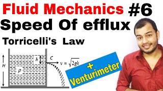
Now come back to where simple experimental setups, we generally do the measuring the flow in a pipe, either in a venturimeter or the orifice meter.
Detailed Explanation
This chunk talks about orifice meters, which measure flow rates in pipes. Orifice meters consist of a plate with a hole that causes a reduction in flow area. The resulting pressure difference across the orifice can be used to calculate discharge using Bernoulli's equation.
Examples & Analogies
Consider orifice meters as the 'traffic cones' of fluid flow. Just like cones direct traffic to reduce jams at intersections, orifice meters control the flow in pipes, allowing engineers to measure and manage the movement of fluids.
Kinetic Energy Correction Factors
Chapter 3 of 9
🔒 Unlock Audio Chapter
Sign up and enroll to access the full audio experience
Chapter Content
That means, for a non-uniform distribution of flow, when you apply this Bernoulli equations, we need to have correction factors if we are using average velocity.
Detailed Explanation
This section highlights the importance of kinetic energy correction factors. Since fluid flow in pipes isn't uniform, the average velocity doesn't accurately represent the flow's kinetic energy. Correction factors are used to account for this discrepancy when using Bernoulli's equations to compute total kinetic energy.
Examples & Analogies
Imagine trying to find the average speed of a car over a bumpy road. The average might not reflect how fast the car was going at different points—just like in fluid flow, the kinetic energy can vary. The correction factors help us understand the flow better.
Define Pressures Associated with Fluid Flow
Chapter 4 of 9
🔒 Unlock Audio Chapter
Sign up and enroll to access the full audio experience
Chapter Content
Fourth part, I will talk about how we can define the three different types of pressures; static, dynamic and stagnation pressures.
Detailed Explanation
In this chunk, the lecturer is about to explain three types of pressures relevant to fluid mechanics: static pressure (pressure exerted by the fluid at rest), dynamic pressure (pressure due to fluid motion), and stagnation pressure (the total pressure when the fluid is brought to rest).
Examples & Analogies
Think of these pressures like the different ways we feel the wind. When standing still (static), we feel pressure), when we move fast (dynamic), we feel wind pressing against us, and when we suddenly stop (stagnation), we feel the accumulated air pressure like a breeze settling down.
Hydraulic and Energy Gradient Lines
Chapter 5 of 9
🔒 Unlock Audio Chapter
Sign up and enroll to access the full audio experience
Chapter Content
Then will come hydraulic and energy gradient lines, that is the basic concept what we will talk about.
Detailed Explanation
This section will introduce hydraulic and energy gradient lines, which are graphical representations of energy losses and flow solutions in pipe networks. These lines help visualize the energy distribution along fluid flow paths.
Examples & Analogies
Imagine hiking down a hill; the energy gradient line shows how steeply you descend, similar to following the energy changes in a fluid as it flows downhill through a pipe.
Applying Bernoulli's Equation in Pipe Flow Systems
Chapter 6 of 9
🔒 Unlock Audio Chapter
Sign up and enroll to access the full audio experience
Chapter Content
Then, I will talk about if we have a pipe flow systems, with a series of pump turbine systems, then how we apply it and how we can quantify different energy mechanical energy also the efficiency to the fluid flow problems.
Detailed Explanation
Here, the lecturer discusses how to apply Bernoulli’s equation to real-world systems involving pumps and turbines. This includes calculating various energy factors and system efficiencies within complex fluid flow setups.
Examples & Analogies
Think of this segment as managing a water park. Just like pumps push water through slides (akin to a pump in a piping system), Bernoulli’s equation helps operators understand and optimize how much energy they need to keep the rides flowing smoothly.
Coefficient of Discharge
Chapter 7 of 9
🔒 Unlock Audio Chapter
Sign up and enroll to access the full audio experience
Chapter Content
Since the Bernoulli equations what we applied, we do not consider the energy loss components.
Detailed Explanation
In pipeline experiments (like venturimeters), actual discharge commonly differs from theoretical discharge due to energy losses, which can be represented through a coefficient of discharge. This coefficient relates the actual flow to theoretical flow calculated by Bernoulli's equation.
Examples & Analogies
Picture a garden hose: it delivers water differently when bent or clogged than expected. The coefficient of discharge adjusts our understanding of flow to account for such real-world conditions.
Application in Fluid Flow Problems
Chapter 8 of 9
🔒 Unlock Audio Chapter
Sign up and enroll to access the full audio experience
Chapter Content
Then we will solve around four fluid flow problems, which are the gate and the engineering service problems will solve, which is part of the Bernoulli equations applications.
Detailed Explanation
This section will propose practical applications and problem-solving using Bernoulli's equation. It emphasizes how to contextually apply theory to real-life hydraulic issues faced in engineering.
Examples & Analogies
Just as students tackle math problems in school to apply what they learn, engineers use Bernoulli’s equations to solve practical issues in fluid dynamics, reinforcing their understanding of concepts.
Concluding Concepts and Real-Life Balance
Chapter 9 of 9
🔒 Unlock Audio Chapter
Sign up and enroll to access the full audio experience
Chapter Content
Then concluding this lecture, we talk about, how our sense of balance is there. So, okay, how it works.
Detailed Explanation
In conclusion, the lecture will address the balance of forces and energy in fluid systems, illustrating the interconnected concepts of Bernoulli's equation to emphasize its significance in engineering.
Examples & Analogies
Think of balance as riding a bicycle; just as you need to maintain your center of gravity to stay upright, engineering fluid flows require a balance of forces to optimize function and efficiency in systems.
Key Concepts
-
Real Fluid Flow Problems: The fundamental utility of Bernoulli's Equation is its ability to model real fluid flows by incorporating correction factors for non-uniformity, such as kinetic energy correction factors. As fluid flows through various devices like orifice and venturi meters, understanding these corrections becomes crucial for accurate discharge measurements.
-
Types of Pressures: The three distinct pressures defined are static pressure, dynamic pressure (or velocity head), and stagnation pressure (sum of the previous two). These pressures are instrumental in calculating fluid flow characteristics and understanding forces acting within fluid environments.
-
Energy Gradient Line & Hydraulic Gradient Line: Both gradient lines visualize the energy perspectives across a fluid system. The energy gradient line represents the total energy including potential, kinetic, and pressure energy, while the hydraulic gradient line excludes the kinetic energy, simplifying certain calculations but still providing crucial insights into fluid behavior.
-
The applications extend through numerous scenarios, including the design of fuel-efficient vehicles, where optimizing drag coefficients has significantly improved consumption rates. Moreover, practical experiments conducted using orifice meters instantiate the application of Bernoulli's principles, illuminating the inherent energy losses versus calculated theoretical values through the understanding of coefficients of discharge.
-
Ultimately, Bernoulli's Equation and its applications remain a cornerstone in fluid mechanics, accomplishing practical, efficient solutions in engineering disciplines today.
Examples & Applications
Example of fuel-efficient cars illustrating how changes in drag coefficient, leveraging Bernoulli's principles, can significantly reduce fuel consumption.
Application of a venturi meter to measure the flow rate in pipelines, demonstrating the practical usage of Bernoulli's Equation.
Memory Aids
Interactive tools to help you remember key concepts
Rhymes
When fluid flows, it’s clear to see, pressure and speed work in harmony!
Stories
Imagine a traveler on a hill (high energy) who flows down to the valley (low energy), following the path of Bernoulli's Equation as they go!
Memory Tools
SPeD (Static, Potential, Dynamic) helps you recall the three types of pressure involved in Bernoulli's Equation.
Acronyms
EGL = Energy Gradient Line tells you all the energy at play in fluid flows!
Flash Cards
Glossary
- Bernoulli's Equation
A principle that relates the pressure, velocity, and elevation of a fluid in steady flow.
- Static Pressure
The pressure exerted by a fluid at rest.
- Dynamic Pressure
The pressure exerted by a fluid in motion, associated with its velocity.
- Stagnation Pressure
The total pressure a fluid would exert if brought to rest.
- Kinetic Energy Correction Factor
A factor that adjusts the average velocity in non-uniform flow for kinetic energy calculations.
- Energy Gradient Line (EGL)
A line that represents the total head (pressure + kinetic + potential) along a streamline.
- Hydraulic Gradient Line (HGL)
A line representing the potential energy (static pressure + elevation) of the fluid, excluding kinetic energy.
- Coefficient of Discharge
A ratio of actual discharge to theoretical discharge taking into account energy losses.
Reference links
Supplementary resources to enhance your learning experience.