
Kinetic Energy Correction Factors
Enroll to start learning
You’ve not yet enrolled in this course. Please enroll for free to listen to audio lessons, classroom podcasts and take practice test.
Interactive Audio Lesson
Listen to a student-teacher conversation explaining the topic in a relatable way.
Introduction to Kinetic Energy Correction Factors
🔒 Unlock Audio Lesson
Sign up and enroll to listen to this audio lesson

Today, we're going to explore kinetic energy correction factors, which are essential when we use Bernoulli's equation. Can anyone tell me why average velocities might not be sufficient in calculating kinetic energy?

I think because fluid flow can be non-uniform, right?
Exactly! That's a great point. The average velocity assumes a uniform flow, but when we have varying velocities across different areas of flow, corrections are needed. We denote this correction factor as alpha (α).

So, how does this correction factor affect our calculations?
Good question! The kinetic energy we calculate from average velocity will underestimate the real energy due to the non-uniform flow. The correction factor helps bridge this gap.
Always remember: the equation for kinetic energy correction factor is a = Kinetic Energy (real) / Kinetic Energy (average).

Is the correction factor the same for all types of flow?
Not quite! For laminar flow, α is typically around 2, whereas for turbulent flow, it varies between 1.04 and 1.11.
To summarize, when calculating kinetic energy in non-uniform flows, we must use a correction factor, α, to ensure accuracy in our fluid mechanics applications.
Understanding Velocity Profiles
🔒 Unlock Audio Lesson
Sign up and enroll to listen to this audio lesson

Let's discuss how the velocity profile within a pipe or channel affects our calculations. Can anyone explain how laminar flow differs from turbulent flow in this context?

Isn't laminar flow smooth, while turbulent flow is chaotic and has swirling motions?
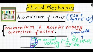
Yes, that's correct! Laminar flow has a parabolic velocity profile, while turbulent flow exhibits a flatter velocity profile near the center. This difference leads to different correction factors.
So, if turbulence increases, does the correction factor also increase?
Usually, the correction factors for turbulent flow are lower than for laminar, which reflects the energy losses in the flow due to turbulence.
Remember, with non-uniform flow, we have different velocities relative to their positions, which is key to understanding correction factors.
Can we visualize this difference somehow?
Absolutely! Imagine a still pond representing laminar flow versus a turbulent river. The chaos of the river represents how velocity varies significantly with distance, requiring correction factors.
In summary, when analyzing flow profiles, the nature of the flow directly impacts our kinetic energy correction factors, essential for accurate calculations.
Practical Applications of Kinetic Energy Correction Factors
🔒 Unlock Audio Lesson
Sign up and enroll to listen to this audio lesson
Now let's reflect on the importance of kinetic energy correction factors in real hydraulic systems. Why do you all think this understanding is important?
It could help in designing more efficient systems, right?
Exactly! When designing pipes, channels, or pumps, accounting for these factors can lead to better efficiency and reduced energy costs.
If we ignore these factors, what could happen?
Ignoring correction factors could lead to underestimating energy needs, resulting in insufficient pump horsepower or larger, inefficient systems!
It's crucial to integrate these factors in our design and evaluation protocols. Remember, these small adjustments can significantly enhance system performance.
So, by applying these concepts, we can improve overall system designs?
Absolutely! In summary, always remember to apply kinetic energy correction factors to ensure your hydraulic systems perform optimally. They make a big difference!
Introduction & Overview
Read summaries of the section's main ideas at different levels of detail.
Quick Overview
Standard
Kinetic energy correction factors account for the discrepancies in kinetic energy calculations when using average velocity in non-uniform flow scenarios. This section highlights how these factors are crucial for accurately applying the Bernoulli equation in fluid dynamics, addressing different flow types, and ensuring effective design in fluid systems.
Detailed
Kinetic Energy Correction Factors
This section focuses on the concept of kinetic energy correction factors, a vital consideration when applying the Bernoulli equation to real fluid flow problems. In fluid mechanics, the flow is rarely uniform, especially in pipelines and channels where disturbances can cause variations in velocity profiles. The equations derived, such as Bernoulli's equation, assume ideal conditions that may not reflect actual scenarios. Therefore, when using average velocity to compute kinetic energy, we must consider correction factors to account for the non-uniform velocity distribution. These factors, denoted as B1 (alpha), help amend the discrepancies observed between theoretical and actual kinetic energy outputs during flow analysis.
For laminar flow, this correction factor can be approximated to be around 2, while for turbulent flow, it ranges approximately from 1.04 to 1.11. Understanding and calculating the appropriate kinetic energy correction factor is essential for accurate fluid dynamics predictions, influencing the design and efficiency of hydraulic systems.
Youtube Videos


Audio Book
Dive deep into the subject with an immersive audiobook experience.
Understanding Kinetic Energy Correction Factors
Chapter 1 of 3
🔒 Unlock Audio Chapter
Sign up and enroll to access the full audio experience
Chapter Content
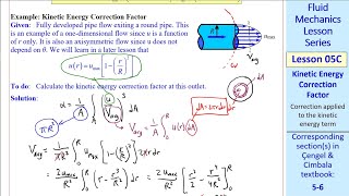
In fluid flow problems, the velocity distributions are often non-uniform. This means that we cannot simply use the average velocity to compute the kinetic energy. To accurately calculate the kinetic energy for such cases, we need kinetic energy correction factors, denoted as α.
Detailed Explanation
In fluid mechanics, we frequently encounter situations where fluid velocity is not evenly distributed across a flow area. For example, in a pipe, the velocity is maximum in the center and decreases towards the walls, creating a parabolic velocity profile. Due to this, if we calculate kinetic energy using just the average velocity, we will misrepresent the actual kinetic energy present in the fluid. To correct for this, we introduce the kinetic energy correction factor α, which allows us to adjust our calculations based on the actual velocity distribution.
Examples & Analogies
Think of it like measuring the average temperature in a room with a heater. If the heater is placed in the corner, the average temperature measured closer to the center may not reflect the actual comfort level in all parts of the room. Similarly, in fluid flow, using the average velocity without considering how the speed changes can lead to inaccurate energy calculations.
Calculating Kinetic Energy Correction Factor
Chapter 2 of 3
🔒 Unlock Audio Chapter
Sign up and enroll to access the full audio experience
Chapter Content
For incompressible flow, the correction factor α can be integrated over the area to find its value. The average velocity V is derived from the velocity profiles and can be represented for fully developed laminar flow and turbulent flow.
Detailed Explanation
To determine the value of α, we mathematically integrate the kinetic energy across the flow area. For fully developed laminar flow, it has been found that α equals 2. In turbulent flow, α ranges from 1.04 to 1.1. This means that, depending on the flow type, the kinetic energy derived from just using average velocity will need to be multiplied by these factors to get an accurate representation of actual kinetic energy in the fluid.
Examples & Analogies
Consider a basketball team where some players are fast runners, and others are not. If you were to calculate the team's average speed during a game, you would miss how much faster the quick players could help in scoring points. Just like the basketball players contribute differently to the team’s performance, different parts of the fluid flow contribute to the overall kinetic energy. The correction factors account for these variations.
Importance of Kinetic Energy Correction Factors
Chapter 3 of 3
🔒 Unlock Audio Chapter
Sign up and enroll to access the full audio experience
Chapter Content
Kinetic energy correction factors are crucial in applications of the Bernoulli equation. They ensure that when we use average velocity for energy calculations, we consider the actual velocity distribution of the fluid, thereby leading to more accurate results.
Detailed Explanation
When applying the Bernoulli equation, neglecting the variations introduced by velocity distributions can result in significant errors, especially in design and analysis tasks for engineers. The kinetic energy correction factor thus plays a vital role in ensuring that the principles derived from Bernoulli's equation accurately reflect real-world fluid behaviors. By using these factors, we can derive more precise solutions to fluid flow problems, whether in pipe systems, channels, or other applications.
Examples & Analogies
Imagine trying to calculate the speed of a river based solely on one point measurement. If you consider only the area where the current is slow, you'd miss the rapid waters in other places that dramatically affect how fast the river flows overall. To get a full picture, you need to account for those variations – just as we do with kinetic energy correction factors.
Key Concepts
-
Importance of Kinetic Energy Correction Factors: Understanding how kinetic energy correction factors adjust kinetic energy calculations for real fluid flow conditions.
-
Velocity Profiles: How laminar and turbulent flow velocity profiles affect kinetic energy calculations and the associated correction factor.
Examples & Applications
In laminar flow, a correction factor of approximately 2 is used for calculating kinetic energy.
For turbulent flow in pipes, correction factors range from 1.04 to 1.11, ensuring accurate energy assessments in varied flow conditions.
Memory Aids
Interactive tools to help you remember key concepts
Rhymes
Flow can be smooth or have a swirl, for energy correction, give it a whirl!
Stories
Imagine a smooth river (laminar flow), where peace reigns, but then it rushes into rocky rapids (turbulent flow), twisting and turning, needing corrections for true energy measure!
Memory Tools
Use 'K-C-F' for 'Kinetic Correction Factor' to remember to adjust your energy calculations!
Acronyms
Remember 'TLC' - Turbulent = Lower Correction, Laminar = Higher Correction.
Flash Cards
Glossary
- Kinetic Energy Correction Factor (α)
A factor applied to adjust kinetic energy calculations for non-uniform velocity distributions in fluid flow.
- Laminar Flow
A type of flow characterized by smooth and orderly motion where fluid particles move in parallel layers.
- Turbulent Flow
A type of flow characterized by chaotic and irregular fluid motion, resulting in mixed layers and increased velocity fluctuations.
- Bernoulli Equation
An equation that describes the conservation of mechanical energy in flowing fluids.
Reference links
Supplementary resources to enhance your learning experience.