
Fluid Flow Problems Related to Bernoulli Equations
Enroll to start learning
You’ve not yet enrolled in this course. Please enroll for free to listen to audio lessons, classroom podcasts and take practice test.
Interactive Audio Lesson
Listen to a student-teacher conversation explaining the topic in a relatable way.
Introduction to Bernoulli's Equation
🔒 Unlock Audio Lesson
Sign up and enroll to listen to this audio lesson

Welcome everyone! Today we will explore Bernoulli's equation and its applications in fluid mechanics. Can anyone tell me why this equation is important?

I think it helps us understand how fluids flow in different situations?
Exactly! Bernoulli's equation simplifies complex fluid flow problems, which significantly contributed to advancements during the industrial revolution. It aids in designing pipe flows and open channels.

When was it introduced?
It was introduced in 1752 by Daniel Bernoulli. Its relevance continues in modern fluid mechanics.
To remember its significance, let's use the acronym B.E.E. – Bernoulli’s Equation Equals flow understanding.

That's a great way to remember!
Glad you like it! Now, let's dive into its applications.
Kinetic Energy Correction Factors
🔒 Unlock Audio Lesson
Sign up and enroll to listen to this audio lesson

Next, let's discuss kinetic energy correction factors. Why do you think we need to correct the kinetic energy in fluid flow?

Maybe because the flow isn't uniform?
Exactly! In reality, fluid flow is often non-uniform, leading to variations in velocity distributions. When we compute kinetic energy using average velocity, we need a correction factor, called alpha (α).
How do we calculate this alpha value?
For laminar flow, α is about 2, while for turbulent flow, it ranges from 1.04 to 1.11. This is crucial for accurate energy assessments.
So, we can’t overlook it when using Bernoulli’s equation.
Correct! Always remember, when dealing with energy, account for the kinetic energy correction factor!
Types of Pressure in Fluid Systems
🔒 Unlock Audio Lesson
Sign up and enroll to listen to this audio lesson
Now, let's explore different types of pressure in fluid systems. Can anyone name a type of pressure?
How about static pressure?
Absolutely! Static pressure is the pressure exerted by the fluid at rest. What about dynamic pressure?
That's related to the fluid's motion, isn't it?
Exactly! Dynamic pressure arises from the fluid flow and can be calculated using the kinetic energy term. Lastly, we have stagnation pressure, which is a combination of static and dynamic pressures.
How does stagnation pressure help us?
It allows us to measure the total pressure at a point where the fluid is brought to rest. Very useful in calculating velocities in flows!
Energy and Hydraulic Gradient Lines
🔒 Unlock Audio Lesson
Sign up and enroll to listen to this audio lesson
Let’s take a look at the energy gradient line (EGL) and hydraulic gradient line (HGL). Can anyone explain the difference?
EGL considers all energy types?
Correct! EGL includes potential, kinetic, and flow energy. HGL, on the other hand, only accounts for static pressure and elevation head. Drawing these lines helps visualize energy changes in flow.
And this helps in designing piping systems?
Yes! Knowing how energy changes along a streamline guides engineers in troubleshooting and designing fluid systems.
I see, so they tell us how energy is used or lost as fluid moves.
Exactly! Let's remember E for energy gradient and H for hydraulic gradient!
Applications: Coefficient of Discharge
🔒 Unlock Audio Lesson
Sign up and enroll to listen to this audio lesson
Finally, let's discuss the coefficient of discharge (Cd) used in orifice meters and venturimeters. What is its role?
Does it account for energy losses?
Correct! The coefficient of discharge is the ratio of actual discharge to theoretical discharge. It accounts for losses due to friction and turbulence.
So, if Cd is low, it indicates more losses?
Right! When designing systems, knowing Cd helps us predict how fluids will behave in real situations.
This whole discussion ties back to Bernoulli's equation!
Exactly! Remember, Bernoulli's equation helps simplify our understanding of fluid behavior.
Introduction & Overview
Read summaries of the section's main ideas at different levels of detail.
Quick Overview
Standard
In this section, we delve into the practical applications of Bernoulli's equation in fluid mechanics, focusing on kinetic energy correction factors, pressure definitions, and how to analyze pipe flow systems. The material emphasizes understanding the energy loss in fluid systems and introduces various parameters, such as discharge coefficients, to enhance the application of the Bernoulli equation.
Detailed
Detailed Summary
In this section, we cover the significance of Bernoulli's equation in fluid mechanics and its extensive applications in real-world fluid flow problems. The chapter starts with an introduction to the historical context of Bernoulli's equation, highlighting its role in simplifying fluid flow problems and aiding the design of various hydraulic systems since its introduction in 1752.
Key topics include:
- Applications of Bernoulli's Equation: Understanding how the equation is utilized in different scenarios, including pipe flow, channel flow, and systems with pumps and turbines.
- Kinetic Energy Correction Factors: Addressing non-uniform velocity distributions and their impact on flow calculations, emphasizing the need for correction factors for accurate kinetic energy assessments.
- Pressure Types: Defining static, dynamic, and stagnation pressures, and explaining how they interact within fluid systems.
- Energy Gradient Line and Hydraulic Gradient Line: Introducing concepts used to visualize energy changes within fluid systems.
- Coefficient of Discharge: Clarifying how it accounts for energy lost due to friction and turbulence, enhancing the accuracy of predicted discharge rates from devices like orifice meters and venturimeters.
Through problem-solving examples, the chapter illustrates how to apply these concepts in engineering contexts, particularly for gate and engineering service problems. The conclusion reinforces the theoretical knowledge with practical insights on fluid mechanics.
Youtube Videos


Audio Book
Dive deep into the subject with an immersive audiobook experience.
Introduction to Bernoulli’s Equation Applications
Chapter 1 of 5
🔒 Unlock Audio Chapter
Sign up and enroll to access the full audio experience
Chapter Content
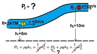
Welcome all of you for this very interesting lecture on Bernoulli Equation and its Applications. Today I will give a very simple way representation of this Bernoulli equation, how we can use it for real fluid flow problems with some correction factors.
Detailed Explanation
In this section, we begin with an introduction to the Bernoulli Equation and its significance in fluid mechanics. The Bernoulli Equation simplifies fluid flow problems, which has historical roots dating back to 1752. Understanding this equation allows engineers to better design systems involving fluid flow, like piping and channel systems. The focus today is on practical applications of this equation, including how to incorporate factors that correct for real-world conditions.
Examples & Analogies
Imagine you are hiking down a hill. If you were to roll a ball down that hill, it would pick up speed due to gravity (just like fluid speeding up due to pressure differences). The Bernoulli Equation helps us predict how fast that ball, or in our case fluid, will flow based on the height of the hill and how wide the path is.
Introduction to Kinetic Energy Correction Factors
Chapter 2 of 5
🔒 Unlock Audio Chapter
Sign up and enroll to access the full audio experience
Chapter Content
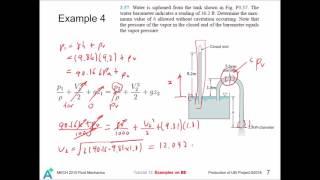
I will talk about kinetic energy corrections factors. For a non-uniform distribution of flow, when we apply this Bernoulli equations, we need to have correction factors if we are using average velocity.
Detailed Explanation
This part of the lecture introduces kinetic energy correction factors, essential for accurately applying the Bernoulli Equation. In real fluid flows, the velocity is often not uniform; it can vary from slow at the edges of a pipe to fast at the center. Because we often use an average velocity in calculations, correction factors help us adjust for the differences in velocity distribution to get a more accurate calculation of kinetic energy.
Examples & Analogies
Think of a crowded stadium, where most people are standing still, but a few are running toward the exit. If you wanted to find out how fast people are leaving the stadium overall, you'd need to consider the runners' speed rather than just average everyone standing still. The kinetic energy correction factor serves a similar purpose in fluid mechanics.
Static, Dynamic, and Stagnation Pressures
Chapter 3 of 5
🔒 Unlock Audio Chapter
Sign up and enroll to access the full audio experience
Chapter Content
I will talk about how we can define the three different types of pressures: static, dynamic, and stagnation pressures.
Detailed Explanation
In this part, we differentiate between static pressure, dynamic pressure, and stagnation pressure. Static pressure is the pressure exerted by a fluid at rest, dynamic pressure is associated with the fluid's motion, while stagnation pressure represents the total pressure when the fluid is brought to a complete stop. It is the sum of static and dynamic pressure, which helps us understand how energy is distributed in flowing fluids.
Examples & Analogies
Imagine you are at a water park. When you dive into a pool, the pressure of the water pressing on you underwater is similar to static pressure. As you swim, the rush of water around you (your speed) relates to dynamic pressure. If you suddenly stopped and sank to the bottom, the total pressure you'd experience would be akin to stagnation pressure, combining both static and dynamic effects.
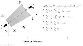
Energy and Hydraulic Gradient Lines
Chapter 4 of 5
🔒 Unlock Audio Chapter
Sign up and enroll to access the full audio experience
Chapter Content
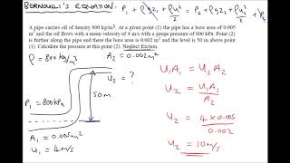
Then we will come to hydraulic and energy gradient lines, that is the basic concept what we will talk about. The energy gradient line represents the total energy of the fluid, while the hydraulic gradient line is related to the pressure and elevation head.
Detailed Explanation
Here, we introduce two important concepts: the energy gradient line and the hydraulic gradient line. The energy gradient line visualizes the total energy (kinetic, potential, and pressure energy) in a flowing fluid system, while the hydraulic gradient line helps in understanding the pressure changes alongside elevation. These lines are crucial for engineers when designing fluid systems, as they indicate how energy diminishes or transforms as fluid moves from one point to another.
Examples & Analogies
Imagine you are observing a river flowing down a hill. The river's total energy at any point relates to how fast it’s moving, how high it is above sea level (potential energy), and how much pressure is exerted by the water. The energy and hydraulic gradient lines would help you visualize this energy balance throughout the course of the river.
Coefficient of Discharge in Orifice Meters
Chapter 5 of 5
🔒 Unlock Audio Chapter
Sign up and enroll to access the full audio experience
Chapter Content
Whenever flow goes through these venturimeter or orifice meter, there will be energy losses. Because of the energy losses, there will be difference between theoretical discharge and actual discharge.
Detailed Explanation
In this chunk, we focus on orifice meters and how they are utilized in measuring fluid discharge. Due to energy losses in real systems—such as turbulence and friction—theoretical calculations using Bernoulli’s Equation often overestimate the discharge. To account for this discrepancy, engineers introduce the coefficient of discharge, which relates actual discharge to theoretical discharge. It is essential to consider this coefficient when designing and analyzing fluid systems.
Examples & Analogies
Think of a toothpaste tube. When you squeeze it, the toothpaste comes out smoothly at first, but if you twist the tube or apply uneven pressure, it may come out irregularly or even stop, showing that energy losses have occurred. The coefficient of discharge helps you predict how much toothpaste (or fluid) actually comes out despite these interruptions.
Key Concepts
-
Bernoulli's Equation: Relates pressure, velocity, and height in fluid dynamics.
-
Kinetic Energy Correction Factor: Accounts for changes in velocity distribution.
-
Types of Pressure: Static, dynamic, and stagnation pressure have distinct roles.
-
Energy Gradient Line (EGL): Represents total energy of fluid flow.
-
Hydraulic Gradient Line (HGL): Reflects static pressure and elevation in a fluid system.
-
Coefficient of Discharge (Cd): Corrects theoretical discharge for real losses in flow.
Examples & Applications
A car's aerodynamic design reduces drag force, showcasing the application of Bernoulli's equation to improve fuel efficiency.
An orifice meter is used in a fluid flow system to measure discharge, where Cd accounts for energy losses due to friction.
Memory Aids
Interactive tools to help you remember key concepts
Rhymes
In fluid flows where pressure gleams, Bernoulli guides like flowing streams.
Stories
Imagine a water slide where the pressure at the top is high. As you slide down, the water speeds up, demonstrating dynamic pressure decreases with height, while total energy remains constant.
Memory Tools
Remember 'E.P.D.' - Energy, Pressure, Discharge for fluid flow understanding.
Acronyms
B.E.E. - Bernoulli’s Equation Equals flow understanding.
Flash Cards
Glossary
- Bernoulli's Equation
A principle that relates pressure, velocity, and height in a flowing fluid.
- Kinetic Energy Correction Factor
A factor used to account for variations in velocity distribution when calculating kinetic energy.
- Static Pressure
The pressure exerted by a fluid at rest.
- Dynamic Pressure
The pressure associated with a fluid's motion, calculated from the velocity of the flow.
- Stagnation Pressure
The total pressure of a fluid when brought to a complete stop, combining static and dynamic pressure.
- Coefficient of Discharge (Cd)
A dimensionless number that represents the ratio of actual discharge to theoretical discharge in fluid flow.
- Energy Gradient Line (EGL)
A line that represents the total energy head of fluid flow along a streamline.
- Hydraulic Gradient Line (HGL)
A line that indicates the pressure head and elevation head in a fluid system, without considering kinetic energy.
Reference links
Supplementary resources to enhance your learning experience.